


|
|
|
Trendline Synthesis - a new music synthesis technique
Posted: 1 January 2016 Revised: 23
October 2024
Abstract. When simulating musical instruments it is often necessary to adjust the tone colour or timbre of existing sound samples, or to produce entirely new ones. Conventionally, this requires the creation of new harmonic spectra to represent the new tone colour, and the modified samples are then generated using additive synthesis. However, creating the desired spectra is time consuming and laborious especially when they comprise many harmonics, and it also requires a lot of skill and experience. Similar parameter-overload problems apply to physical modelling synthesis. So some means is desirable to reduce the labour involved, and the technique of Trendline Synthesis described in this article offers this advantage. It enables a wide range of prototype spectra to be created instantaneously by specifying no more than four parameters for each one, regardless of how many harmonics they might contain. Thus manual intervention is minimal, making the design cycle for a new synthetic sample set much faster, cheaper and more flexible than creating it from recordings of existing instruments or constructing a set of new spectra harmonic by harmonic. Audio recordings are included, showing that Trendline Synthesis can produce convincing aural examples of the four classes of pipe organ tone colour - diapasons (or principals), strings, flutes and reeds. These advantages ensue from the simple means by which a spectral envelope is approximated by a set of trendlines, and for organ pipe spectra it has been found that only two lines are necessary. Because only two parameters are required to define a straight line, it follows that no more than four are needed to define both trendlines in any spectrum and thus the spectrum itself. A novel computer design tool is described which facilitates the process.
Contents (click on the headings below to access the desired section)
Examples of organ pipe trendlines
When simulating musical instruments digitally, instances often arise when it is necessary to rapidly adjust the tone colour of existing sound samples, a process known as voicing in the organ world. Or a simulation might need to be developed from scratch for which no sound samples are available. This can occur when entirely new and 'invented' sounds are required, and in such cases sample sets from an existing instrument cannot be created by definition. Even when samples could be obtained in principle from recordings of a real acoustic instrument, the process of producing a high quality sample set is expensive, labour intensive and the result is inherently inflexible because it is difficult to make other than minor changes. In circumstances such as these it is frequently necessary to create new harmonic spectra to represent the required tone colours, or to modify existing spectra by adjusting their harmonic amplitudes. This too requires a lot of toil. These operations have to be done in the frequency domain because it is impossible to modify the time domain waveforms used in sampled sound synthesis directly. Therefore the new or modified samples have to be generated using additive synthesis operating on the new or modified harmonic spectra. In a real time additive synthesis instrument, this step would take place within the instrument itself.
There is nothing wrong in theory with this approach, and it is a conventional and widely used procedure. However in practice, creating the desired harmonic spectra is time consuming especially when they comprise many harmonics, and it requires a lot of skill and experience. Similar problems apply to physical modelling synthesis, in which a large number of parameters are invariably required to define a particular tone colour. For instance, the Viscount 'Physis' system uses 58 parameters for each simulated pipe tone [5]. So some means is desirable to reduce the labour involved, and the technique of Trendline Synthesis described in this article offers this advantage. It enables a wide range of prototype spectra to be created instantaneously by specifying no more than four parameters for each one, regardless of how many harmonics they might contain. The harmonic amplitudes in the spectra are then converted, again instantaneously and automatically, to time domain wave (PCM) files for exporting to a sound sampler. Loop points can also be computed automatically and embedded in the wave files if desired. Thus manual intervention is minimal, making the design cycle for a new sample set much faster, cheaper and more flexible than creating it from recordings of existing instruments. This article shows how Trendline Synthesis can generate convincing examples of the four classes of pipe organ tone colour - diapasons (or principals), strings, flutes and reeds - each of which only requires four parameters to define the tone colour of the sample. Some audio recordings are included.
All the advantages outlined above follow from the simple means by which a spectral envelope is approximated by a set of trendlines. Any number of lines can be used, but for organ pipe spectra it has been found that only two are necessary. Because only two parameters are required to define a straight line, it follows that no more than four parameters are needed to define both lines in any spectrum, hence the economy and simplicity of the method. It has been found that approximating to a set of harmonic amplitudes in a spectrum by using trendlines results in little change to the tone colour. Such changes as do occur are eclipsed in any case by those which arise naturally between one note and the next in real musical instruments such as the pipe organ.
The novelty of the method relates to simulating the pipe organ, where the use of trendlines to approximate to the spectral envelopes of organ pipes does not appear to have been used previously. Other important aspects include the mandatory representation of power spectra using log-log spectral plots rather than either or both axes (power and frequency) employing linear scales. Only with a log-log plot does the simplicity of the technique emerge in which only two linear trendlines, rather than a multiplicity, are necessary.
Trendline Synthesis in more detail
An earlier article on this site introduced the concept of trendlines to approximate to the spectral envelopes of groups of harmonics in an organ pipe spectrum [1], though it can also be applied to other musical.instruments. The general idea is illustrated at Figure 1.
Figure
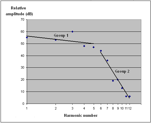
1. Trendlines and spectral groups for a Trumpet pipe
This diagram shows the harmonic amplitudes of an organ Trumpet pipe by Rushworth & Dreaper (blue dots), together with trendlines applied to two easily-identifiable groups of harmonics. The first group includes the low order harmonics having amplitudes comparable with the fundamental, whereas the second group comprises those of higher order which exhibit rapidly diminishing amplitudes. Each trendline was fitted to its group of harmonics using a least-squares procedure. The knee or breakpoint between the two lines, denoting that frequency at which the second takes over from the first, lies near the fifth and sixth harmonics in this case. The previous article [1] demonstrated that spectral groups and trendlines could be identified for each of the four classes of organ tone - diapasons (or principals), flutes, strings and reeds. It also put forward the view that convincing aural reconstructions of the pipe sounds could be achieved using the trendline parameters alone, rather than the usual technique of generating a sound sample by applying additive synthesis to all of the actual harmonics. This view was arrived at after many listening tests, and it represents a considerable simplification when a spectrum contains many harmonics. It was found that approximating to a set of harmonic amplitudes in a spectrum by using trendlines results in little change to the tone colour. Such changes as do occur are eclipsed in any case by those which arise naturally between one note and the next in real musical instruments such as the pipe organ.
This article takes the analysis further into the realm of digital musical instruments. Besides the economies just mentioned, the use of spectral envelopes in the form of trendlines enables a wide range of musical instruments, not just pipe organs, to be simulated readily. Moreover, rapid appraisal and readjustment of the tone colours or timbres becomes possible without having to painstakingly amend some or all of the individual harmonics in a spectrum, even if one knew which ones were relevant. In the particular case of synthesising pipe organ tones digitally, this ability to rapidly 'revoice' an instrument or to create a new one from scratch does not require the expensive, labour intensive and inherently inflexible process of constructing a fixed sample set from recordings of individual organ pipes. This is also an advantage when a new simulation is to be developed for which samples are unavailable, whether of a pipe organ or any other musical instrument. Entirely new and 'invented' sounds can also be generated very easily, and in such cases sample sets from an existing instrument cannot be created by definition. Thus Trendline Synthesis is presented here as a new and flexible music synthesis technique with wide potential application. Although additive synthesis was mentioned above, Trendline Synthesis is not additive synthesis. It merely uses additive synthesis as part of a new process of generating waveform samples which can then be used in a sound sampler. Nevertheless, because a set of harmonic amplitudes is generated as part of the Trendline Synthesis process, these can also be used in a real time additive synthesis sound engine should this be desired.
All the advantages outlined above follow from the simple means by which a spectral envelope is approximated by a set of trendlines. Any number of lines can be used, but for organ pipe spectra it has been found that only two are necessary. A straight line is fully defined using only two parameters - its gradient or slope and its intercept on the vertical axis. This is enshrined in the standard equation of a straight line, written as y = mx + c where m is the gradient and c the intercept (here the vertical axis is taken as the y-direction and the horizontal axis as the x-direction). In practice other convenient parameters can also be used provided they reduce to the form just outlined with two independent (unrelated) values for each line. Thus in this article, a trendline is defined by its slope (specified in decibels per octave - dB/8ve) and the breakpoint or harmonic number at which it ends (for the Group1 line) or at which it starts (for the Group 2 line). The breakpoint is not restricted to lie at an integer harmonic value as it can assume any intermediate point between a pair of adjacent harmonics. Thus two intersecting trendlines can be fully defined on a spectrum plot using just three numerical parameters - their slopes and the common breakpoint (the point of intersection) between them. Using these lines, two sets of harmonic amplitudes can then be generated, each set lying on one of the lines. An example will now be discussed.
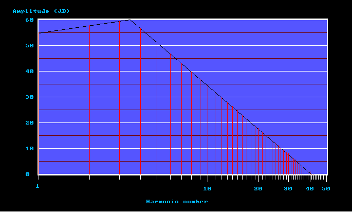
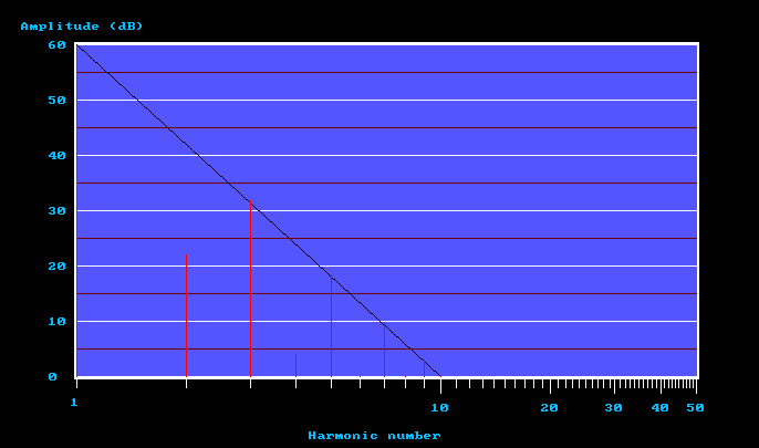
Figure 2. A typical trendline plot
Figure 2 shows a spectrum with two trendlines. The first line has an upwards (positive) slope of 3 dB/8ve and the second has a downwards (negative) slope of -17 dB/8ve. The breakpoint is at a 'harmonic number' of 3.5. The quote marks serve to show that this is, in a sense, a fictitious number because it does not correspond to an actual harmonic, lying as it does between harmonics three and four, but it is more flexible for the breakpoint not to be restricted to integer values. There are 42 harmonics enclosed by the two trendlines. This type of graph is the most important output screen of an interactive design program which I have developed (written in C). The diagram does not correspond to any particular organ tone as it is shown here purely for illustrative purposes, though it relates more closely to the harmonic recipe of a string-toned pipe rather than to any other type. These almost invariably have the upwards slope as shown for the first few (Group 1) harmonics, followed by a steeper descending slope associated with the remaining (Group 2) harmonics. The total number of harmonics, 42, is also typical of pipes with a keen string timbre. Note that the number of harmonics is not required of the user, as this parameter drops out of the process automatically as a consequence of merely having defined the two trendlines. Thus if you want a keener or brighter tone, you simply adjust the lines to give you more harmonics in one region of the spectrum or the other, or both.
So what happens next? What does one do with this picture? It has already been stated that it is only necessary for the user to specify the slopes of the two lines and their breakpoint, that is, to input just three numbers. The screen then appears and harmonics are drawn in automatically, as shown by the red lines in the diagram, and their amplitude values are saved to a file in case one wants to call up a particular spectrum again or for other purposes. These values are also used to generate a Windows wave file by additive synthesis (a standard PCM file with a WAV extension) which can then be auditioned in a sound sampler or wave editor. For this to happen, loop points are created automatically so that the sound lasts for as long as the user wishes. The same looped WAV file can also be imported into one of many external rendering engines such as a software synthesiser or an existing digital organ system, when other articulation parameters such as attack and release envelopes will be added to complete the voicing of the sample.
Note the use of a log-log spectrum plot in which the quantities on both axes are represented logarithmically. This is essential, otherwise the best-fit spectral envelopes turn out to be curves rather than straight lines and more parameters would therefore be required to specify them as (for example) polynomials. Although not directly relevant to this article, it is of interest that the ear and brain process both the amplitude and frequency of sounds logarithmically. It is also not without interest that the simple straight line representation of spectra at the heart of Trendline Synthesis is capable of producing results which satisfy the ear. Therefore there might be implications here for the neural mechanisms of musical perception which were drawn out in the earlier article [1].
Examples of organ pipe trendlines
Although the process of designing sounds using trendlines is essentially simple provided one has the computer-based tools available, it will probably be difficult for a novice to get the sounds s/he wants at first. Some practice is required, and in this respect the technique is no different to any other form of musical instrument synthesis, and indeed to the art of voicing real organ pipes. It is also helpful, if not essential, to have as much experience as possible of what organ pipe spectra look like. This being so, we now look at some specific examples of trendline plots for each of the four classes of organ tone - diapasons (or principals), strings, flutes and reeds - to give a flavour of what the design process entails.
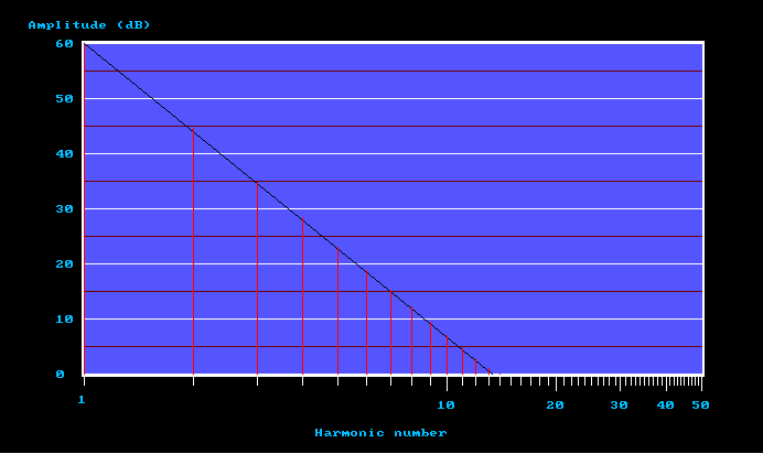
Figure 3 is a plot which generates an Open Diapason tone. It relates to a pipe in the middle of the organ key compass, around middle F sharp, and this is true of all the examples to be discussed. This is an important point since the spectrum of organ pipes varies systematically across the compass as a result of the varying scales of the pipes (scale is a measure of cross-sectional area to length). Thus it is usually not possible to use the same spectrum or harmonic recipe, and thus the same trendline parameters, across the entire compass. Scaling is discussed in more detail later in the article The parameters of the plot were chosen to produce the somewhat subdued, dignified diapason tone typical of a British organ of the first half of the twentieth century rather than that of the brighter and more zestful principals of a German or Dutch instrument.
Figure 3. Trendline plot for an Open Diapason
There are 13 harmonics, all of which lie on the same descending line. This picture was generated using the following parameter set:
Breakpoint at harmonic number: 1 Slope of Group 1 trendline: -16 dB/8ve Slope of Group 2 trendline: -16 dB/8ve
The use of a breakpoint at the first harmonic effectively collapses the Group 1 spectral region and its trendline to nothing, but it is still necessary to specify its gradient to satisfy the syntax of the design program. Thus in practice we are only using a single trendline here to generate the sound of this particular Open Diapason, which demonstrates the economy and efficiency of Trendline Synthesis as a means of designing musical sounds.
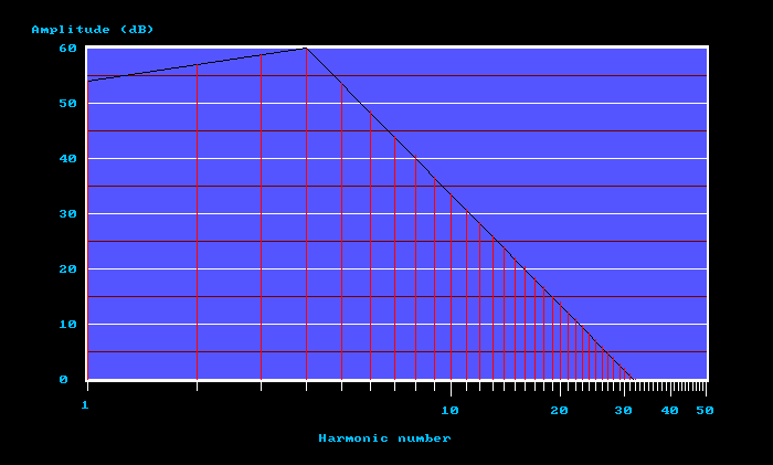
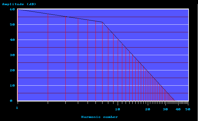
Figure 4 shows a trendline plot for a keen-toned string pipe of the genre often called a Viol d'Orchestre. As before, the spectrum corresponds to the middle region of the key compass.
Figure 4. Trendline plot for a Viol d'Orchestre
There are 32 harmonics, distributed within the regions enclosed by two trendlines. This picture was generated using the following parameter set:
Breakpoint at harmonic number: 4 Slope of Group 1 trendline: +3 dB/8ve Slope of Group 2 trendline: -20 dB/8ve
Figure 5 shows a trendline plot for a stopped flute pipe of the genre often called a Stopped Diapason. This is an unfortunate misnomer as the tone has nothing of the qualities of any other sort of diapason because the pipe has a flute-like tone. The presence of the stopper causes the even-numbered harmonics of the real organ pipe to be suppressed relative to the odds, giving the pipe a characteristically hollow, 'woody' sound for reasons explained in reference [2]. In the design program used here, even harmonic suppression is achieved by introducing a fourth parameter. As before, the spectrum corresponds to the middle region of the key compass.
Figure 5. Trendline plot for a Stopped Diapason
There are 9 harmonics, some of which have negligible amplitudes. As with the Open Diapason, only one trendline is used in effect, this being achieved by specifying a breakpoint at the first harmonic in the same way as before. This picture was generated using the following parameter set:
Breakpoint at harmonic number: 1 Slope of Group 1 trendline: -18 dB/8ve Slope of Group 2 trendline: -18 dB/8ve Even harmonic suppression: 20 dB
Note the extra parameter introduced here which suppresses the even-numbered harmonics relative to the odds by the specified amount. (When using the trendline design program this parameter always has to be given a value, and in the previous cases it was merely set to zero).
Two reed tones are presented here, a Trumpet and a Clarinet. Note these are designed as versions of these sounds familiar to those in the organ world rather than representing the eponymous brass and woodwind instruments. Although there are some passing similarities, the two types of tone (organ and orchestral) are more often characterised by their differences.
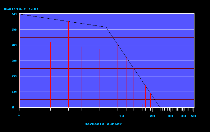
Figure 6 shows a trendline plot for a Trumpet pipe having a fairly bright, assertive and brassy tone. In an organ it might attract a name such as Fanfare Trumpet. As before, the spectrum corresponds to the middle region of the key compass.
Figure 6. Trendline plot for a Trumpet
There are 37 harmonics, distributed within the regions enclosed by two trendlines. This picture was generated using the following parameter set:
Breakpoint at harmonic number: 7 Slope of Group 1 trendline: -3 dB/8ve Slope of Group 2 trendline: -22 dB/8ve Even harmonic suppression: 0 dB
The 'even harmonic suppression' parameter, introduced for the Stopped Diapason above, is again included though it had no effect in this case as it was set to zero.
Figure 7 shows a trendline plot for a Clarinet pipe. It probably inclines more towards the somewhat thin and penetrating tone of a Corno di Bassetto or even a Krumhorn rather than the smoother, more reticent type of Clarinet often encountered. As before, the spectrum corresponds to the middle region of the key compass.
Figure 7. Trendline plot for a Clarinet
There are 23 harmonics, distributed within the regions enclosed by two trendlines. This picture was generated using the following parameter set:
Breakpoint at harmonic number: 7 Slope of Group 1 trendline: -3 dB/8ve Slope of Group 2 trendline: -30 dB/8ve Even harmonic suppression: 15 dB
As with the Stopped Diapason, the 'even harmonic suppression' parameter plays an important role here. Note how qualitatively similar the trendline structure is to that of the Trumpet, the only numerical difference being the somewhat more rapid fall-off for the Group 2 harmonics. But it is mainly the introduction of even harmonic suppression which makes the Clarinet sound so utterly different to the Trumpet.
At this point it might be appropriate to listen to what these examples actually sounded like when the synthesised samples were imported into a sound sampler. The processes required to generate them were described above, but to recapitulate the following steps were involved:
1. Design the trendline spectra on-screen as just described.
2. Using the harmonic amplitudes thus defined, generate samples (wave files) at the desired frequency (defined by MIDI Note Number) for each tone using additive synthesis. Having input the Note Number this is done automatically by the design program - there is no messing about trying to read off the harmonic amplitude values using a cursor, so it is an almost instantaneous process. The harmonic amplitudes are also saved in a separate file for later use if required.
3. Add loop points and embed them in the sample files (the loop points are also identified automatically by the design program).
4. Export the samples to an external sound sampler.
The following mp3 file contains the five examples discussed above and in the same order - Open Diapason, Viol d'Orchestre, Stopped Diapason, Trumpet and Clarinet. Multiple but slightly different instances of each of these tones were generated to simulate the scaling of the corresponding organ pipes across the keyboard, as discussed in more detail below. Additionally, voicing parameters were applied in the sampler itself to simulate proper attack and release envelopes, volume levels and the other necessary features of real organ pipe sounds. Thus each tone is represented as a complete organ stop in the sampler, and the hymn tune 'Moscow' is played on each one in turn. The two reed examples are played as solos accompanied by one of the flue stops so that the tones can be better appreciated.
I find it remarkable that such a wide range of tones can be obtained merely by varying the four parameters of so simple a model, and to my mind it might be saying something about how the ear and brain perceive musical sounds. This idea was developed further in the earlier article [1].
We now come to some additional issues which go beyond synthesising the samples themselves. None of them are specific to Trendline Synthesis because they are common to any other method of generating synthetic samples, so they will not be discussed in excessive detail. Scaling is one of these topics. This is a complex subject and further information can be found elsewhere on this website, for example at reference [2] (see the section entitled Pipe Scales). Briefly, the scale of a cylindrical organ pipe is the ratio of its diameter to its length. Constant scale means that the ratio remains the same across all the pipes which constitute an organ stop, but this is never used. If it were used, the pipes would get too narrow towards the middle and treble end of the key compass. In this case, not only would the overly-narrow pipes eventually cease to emit enough acoustic power but they would sound thin and shrill on account of the excess of harmonics they radiate. This would happen because the number of harmonics emitted by an organ pipe depends on its cross-sectional area, with narrower pipes emitting more harmonics and vice versa. Therefore a variety of non-constant scaling laws is used in which the variation of pipe diameter does not follow the same mathematical progression which governs pipe length. Ascending the key compass from the bass end, pipe length halves every octave (every twelfth note) but pipe diameter reduces more slowly. Typically, the diameter halves every sixteenth note or so for cylindrical flue pipes, with the result that they remain progressively wider as they ascend the compass than they would if constant scaling were used. Thus the effect of scaling is to reduce the number of harmonics which the treble pipes emit and to simultaneously increase the acoustic power which they radiate. Conversely, the bass pipes are narrower (relative to the middle of the key compass) than they would be if constant scaling were used, meaning that they have less of a tendency to overwhelm those higher up the keyboard. They also emit somewhat more harmonics than they otherwise would.
To create a complete synthetic organ stop, multiple samples have to be generated so that they can be scaled across the key compass just as the pipes themselves are scaled in a pipe organ. Desirably, a separate sample should be provided for each note rather than 'stretching' a single sample across a group of adjacent notes, or interpolating the waveforms between two adjacent samples which might be spaced widely across the key compass. Both of these 'short cut' techniques are used often in commercial digital musical instruments. Therefore the spectra for the multiple samples generated for a given simulated organ stop also have to be scaled or 'shaded' to produce the same subtle variation of tone quality across the keyboard as pipe scaling does in a pipe organ. In other words, the same spectrum cannot be used to generate a complete set of samples for realistic simulation of a given organ stop. Because more harmonics are required towards the bass, this has to be reflected in the spectra and hence in the trendline parameters for the corresponding sample files. Towards the treble the reverse applies. Achieving this is a matter of considerable subtlety and it requires some practice and experience to get it right. A good indication of what is required can be found by examining real organ pipe spectra at various points across the keyboard, as it is not something which can be captured in a simple equation or for which simple instructions can be given. To use an appropriate pun, scaling is an example of 'sound design', and it separates the better digital musical instruments (and their tonal designers) from the rest.
How many samples are required for each simulated stop? As mentioned above, ideally there should be one sample per note, just as a pipe organ has one pipe per note, with the trendline parameters for each sample being shaded appropriately across the compass. This is no different to creating a sample set based on recordings of real pipes, in which there should ideally be an independent sample for each note of each stop. However, applying the individual shadings to the trendline parameters is a very much quicker process than laboriously recording, denoising and otherwise preparing a sample set made from acoustic recordings of the pipes.
A more recent article on this site discusses the scaling of synthetic samples in detail [4].
Any synthetic sample when first generated has none of the random variations which can sometimes be heard in real organ pipe sounds, whether it be generated using Trendline Synthesis or any other method. Such variations include small changes in tone quality from note to note, and slight real-time perturbations in amplitude and frequency while a note is sustained. However in my opinion these, and the subject itself, often take on an unreal and bizarre Emperor's New Clothes quality in some quarters. Sometimes an exaggerated posture seems to be adopted that, because a particular organ system is capable of rendering the variations, then you are darn well going to have to listen to them! (Much the same attitude surfaces regarding equally exaggerated attack and release transients). So instead of allowing the issue to develop a conflated life of its own it is better to focus on reality. As an example, recently I heard an organ built in 1858 and meticulously restored by a master organ builder (Mander), in which there was absolutely no random variation detectable in the notes comprising an Oboe solo. The same sounds could quite easily have been generated by the simplest digital sample looped over just a single cycle of the waveform, and it would have been impossible to tell the difference! Therefore it seems to me that certain sections of the digital organ community exaggerate the real importance of randomness, perhaps because so many sample sets recorded from organs are in fact of poor quality because the pipe organ itself was not in good condition. There is no doubt that some sample sets are unsatisfactory, and of course random variations in such cases will often be pronounced and impossible to ignore. But this is unacceptable, particularly in those cases where one has to pay for them. Minutely simulating an organ whose pipes, action and winding system are in poor condition is perverse. Life is too short to waste time, effort and money in this way. Even if randomness can be heard on a pipe organ, it is frequently only at short range. At realistic listening distances and in reasonably reverberant conditions the variations frequently cannot be discerned. Similarly, the majority of organ music does not consist of homophonic single-note solos of long duration - it is polyphonic and moves faster, and it then becomes impossible to detect the random variations of each note even if they are present.
Nevertheless there is some benefit to be gained from injecting a sensible measure of randomness into a sample set which is generated purely synthetically. One simple way to do this is to vary the deterministic and strongly-correlated harmonic amplitudes initially resulting from Trendline Synthesis from note to note across the keyboard. Randomising the amplitudes of individual harmonics within a certain range, say up to ± 5 dB of the values initially calculated, can be done automatically and very easily. The resulting spectra then have some of the amplitude scatter which real pipe spectra exhibit from note to note. However it is seldom necessary to do this because scatter will be imposed naturally on the spectra of all the samples when they are replayed using loudspeakers in any room, owing to the reflections occurring at the room boundaries. Only when listening using headphones will this not happen. Another technique is to modulate the instantaneous amplitude and frequency of each sample slightly using a random number sequence while the sample is sounding. This can either be done in real time by the sampler if it is capable enough, or the variations can be impressed off-line on the samples before they are imported into the sampler. The sampler can also be programmed to apply one-off small changes to the amplitude and frequency of each sample - note that this is additional to the real time variations just mentioned. The frequency variations reflect the fact that no real musical instrument will ever be perfectly in tune within itself. Yet another option is simply to add wind noise.
In addition, audible attack and release transients can be added, though not to all samples otherwise the effect is identifiably unreal. An example of the way I synthesise attack transients is described elsewhere on this site in reference [3] (see the section entitled Attack Transients).
Trendline Synthesis is an example of spectral envelope processing in which the envelopes are of the simplest form possible - straight lines. Formally, the envelope is represented in piecewise linear fashion. It has been found that only two trendlines are required to characterise the harmonic amplitude envelopes of most, if not all, organ pipe spectra in the four categories of diapasons (or principals), strings, flutes and reeds. This means that no more than four parameters are required to define any organ tone synthetically, regardless of how many harmonics it contains, because a straight line is specified by two numbers. The harmonic amplitudes in the synthetic spectrum lie on the trendlines, therefore it is trivially easy to compute a complete synthetic spectrum, and this can be transformed into the time domain by applying additive synthesis (the real discrete inverse Fourier transform). It has been found that a very wide range of prototype organ tone colours can be generated in this way, that is by varying only a few parameters rather than attempting to create a complete spectrum each time by laboriously specifying the amplitude of each harmonic, or by attempting to modify the large number of parameters involved in physical modelling. A computer design tool has been developed to test these ideas which generates wave samples for importing directly into a sound sampler.
It is only possible to use a piecewise linear approximation to the spectral envelopes of organ pipe sounds when the spectra are mapped into a log-log domain having logarithmic axes for both amplitude and frequency. Otherwise the trendlines become curved, requiring higher-order polynomials or other nonlinear functions to represent the approximated envelopes. It is not known why this happy simplification occurs, but it might be related to the fact that the ear and brain also process amplitude and frequency logarithmically. This might have evolved in response to natural music-like sounds arising in the environment, such as within the vocal tracts of animals and humans. Independently of such speculation however, this article has shown unequivocally that the simple straight line representation of spectra at the heart of Trendline Synthesis is capable of producing results which satisfy the ear, therefore there might nevertheless be implications here for the neural mechanisms of musical perception. Perception involves pattern recognition, the process of identifying incoming audio information by assigning it to one of a variety of classes such as the type of musical instrument or organ pipe which generated it. Machine recognition in artificial intelligence often employs piecewise linear feature extraction or classification (such as the nearest neighbour classifier), and there is no a priori reason in principle why brains should not employ similar mechanisms.
1. "Some novel observations on organ pipe sounds and their frequency spectra", an article on this website, C E Pykett, November 2015.
2. "How the flue pipe speaks", an article on this website, C E Pykett, November 2001.
3. "Creating sample sets for digital organs from sparse data", an article on this website, C E Pykett, February 2013.
4. "Scaling synthetic samples across the key compass", an article on this website, C E Pykett, March 2016.
5. "Introducing Deep Machine Learning for Parameter Estimation in Physical Modelling", Zinato et al, Proc. 20th Conference on Digital Audio Effects, Edinburgh UK, September 2017.
A subsequent paper took the approach further:
|