


|
|
|
Scaling synthetic samples across the key compass
Colin Pykett
Posted: 10 March 2016 Last revised: 10 March 2016 Copyright © C E Pykett 2016
Abstract. When simulating musical instruments using synthetic waveform samples it is necessary to adjust or 'scale' the samples across the key compass to imitate the variations in timbre or tone quality which occur in the real acoustic instruments. In the pipe organ, each pipe comprising a stop is scaled (dimensioned) deliberately to encourage its timbre and loudness to remain subjectively of a piece across the rank. For example, cylindrical pipes of diapason (principal) tone quality are often scaled so that their diameters halve at the interval of a major tenth, in contrast to their speaking lengths which perforce must halve every octave.
This article shows how scaling laws affect the harmonic spectra of the pipes by representing each spectrum as two trendlines. Only three numbers are required to define the trendlines, namely their point of intersection and their slopes, which is considerably fewer than attempting to specify a spectrum using the amplitudes of its constituent harmonics. An additional reason for using a trendline approximation to represent a spectrum, rather than using the harmonics themselves, is that no two pipes of any organ stop sound exactly the same in terms of their timbres. Moreover, the tone colour of any one pipe varies significantly at different points in the building owing to standing wave effects. This intrinsic variability enables trendlines to capture the essentials of spectra which are subject to these perturbations, because the lines themselves are not influenced as strongly as are the individual harmonics by random variations - the lines tend to 'iron out' the scatter among the harmonics.
Variations in each of the three trendline parameters for a real diapason stop across the key compass are presented and explained in terms of its scaling. The results suggest how to scale the spectra of a synthetic sample set upwards towards the treble and downwards towards the bass to represent a complete and consistently-scaled diapason rank, and it is shown how wave samples can be derived from the trendline parameters for use in a sound sampler. It is also shown how the data can be used to generate similar sample sets for a chorus of diapason stops at different pitches which are properly scaled in relation to the unison rank, just as in a pipe organ.
The method is general and it can therefore be applied when simulating the other classes of organ tone (flutes, strings and reeds) as well as other musical instruments.
Contents (click on the headings below to access the desired section)
Spectrum variations across the key compass
Generating the synthetic samples
When simulating musical instruments digitally, instances often arise when it is necessary to generate sounds synthetically as opposed to recording (copying or sampling) them from real acoustic instruments. Frequently a simulation needs to be developed from scratch when no real sound samples are available. This can occur when entirely new and 'invented' sounds are required, and in such cases sample sets from an existing instrument cannot be created by definition. An example arises when creating sample sets to simulate old organs which either no longer exist or whose pipework has been badly disturbed [1]. Even when samples could be obtained in principle from recordings of real pipes, the process of producing a high quality sample set is labour intensive and expensive, yet the result is inherently inflexible because it is difficult to make other than minor changes. This is a straitjacket which stifles creativity and it illustrates a further disadvantage of this form of sampled sound synthesis. For these reasons it is often necessary to create synthetic samples using a modelling approach. There are basically two modelling techniques in common use - additive synthesis and physical modelling. Both have their pros and cons, and both can lead to acceptable results - or not - with the degree of success depending on the skill of the tonal designer.
In additive synthesis, a waveform sample is created from the harmonic spectrum representing the required tone colour. Thus the sounds are first of all designed in the frequency domain, because it is impossible to 'voice' or modify the time domain waveforms used in sampled sound synthesis directly. Therefore the new or modified synthetic sample waveforms have to be generated using additive synthesis operating on the new or modified harmonic spectra. In a real time additive synthesis instrument this step would take place within the instrument itself. However such instruments are rare, and it is more usual to synthesise the waveform samples offline before importing them into a sound sampler. An advantage of additive synthesis is that exact reconstruction of the desired timbres or tone colours can be achieved if the spectra are correct, and if they are not then voicing is readily accomplished in principle (though it can be difficult in practice, requiring a lot of skill and experience). In physical modelling, mathematical models are set up of the aerodynamic and acoustic processes in organ pipes which run when notes are keyed. The models generate synthetic audio waveforms which can be regarded as 'samples' in the context of this article. A problem here is that the models are only approximate because the acoustics of organ pipes is still not fully understood [2]. Also the models have to be as simple as possible if real time simulation is required, rather than running more complex ones offline to generate the corresponding waveforms beforehand.
Regardless of how they might be produced, when designing synthetic waveforms a major problem arises with scaling them across the key compass. Scaling refers to the subtle changes in tone colour which occur across any rank of organ pipes, and these have to be incorporated into synthetic waveforms also if they are to sound realistic. This happens automatically when samples are copied from a pipe organ, provided that many are recorded across the keyboard for each stop. In theory it ought to happen automatically with physical modelling as well provided values are assigned correctly to a sizeable array of parameters for each simulated pipe, describing both the pipe itself and the way it is voiced and winded. In practice there are limits as to what can be achieved however. Similarly, it is not obvious how the effects of scaling can be reflected in the harmonic spectra of the sounds when using additive synthesis. Thus when scaling modelled synthetic samples it is necessary for the designer to draw on guidance from his/her aural experience, and it tends to be a rather hit and miss affair as to whether the results turn out to be realistic or not. Most readers will know that scaling is essential because it is not possible to use the same pitch-shifted waveform across the entire keyboard - the corresponding tone colour might well sound fine in the middle of the compass but elsewhere it becomes unconvincing. Some maintain that the holy grail of synthetic sample set production is to be able to generate a complete and convincing suite of waveforms across the keyboard from just a single prototype - I can say this with some certainty because of the number of enquiries on this subject I have received over the years. Although this represents a goal which is not always attainable, it can be facilitated using the techniques described in this article which show how the harmonic spectra of organ stops vary systematically across the key compass.
Scaling in pipe organs is a formidably complex subject and for reasons of brevity further information should be sought elsewhere. An introductory review can be found in another article on this website [3] (see the section entitled Pipe Scales). Briefly, the scale of a cylindrical organ pipe is the ratio of its diameter to its length. Constant scale means that the ratio remains the same across all the pipes which constitute an organ stop, but this is never used. If it were used, the pipes would get too narrow towards the middle and treble end of the key compass. In this case, not only would the overly-narrow pipes eventually cease to emit enough acoustic power but they would sound thin and shrill on account of the excess of harmonics they radiate. This would happen because the number of harmonics emitted by an organ pipe depends on its cross-sectional area, with narrower pipes emitting more harmonics and vice versa. Therefore a variety of non-constant scaling laws is used in which the variation of pipe diameter does not follow the same mathematical progression which governs pipe length. Ascending the compass from the bass end of the keyboard, pipe length halves every octave (every twelfth note) but pipe diameter reduces more slowly. Typically the diameter halves at the interval of a major tenth, that is at every sixteenth successive note, for cylindrical flue pipes of diapason (principal) tone. This results in them remaining progressively wider as they ascend the compass than they would be if constant scaling were used. Thus the effect of scaling is to reduce the number of harmonics which the treble pipes emit and to simultaneously increase the acoustic power which they radiate. Conversely, the bass pipes are narrower (relative to the middle of the key compass) than they would be with constant scaling, meaning that they have less of a tendency to overwhelm those higher up the keyboard. They also emit somewhat more harmonics than they otherwise would.
This behaviour has to be simulated when synthetic waveforms are generated, no matter how the modelling is done. To create a complete synthetic organ stop, multiple waveforms have to be created so they can be scaled across the key compass just as the pipes themselves are scaled in a pipe organ. Desirably a separate waveform should be provided for each note, though some digital instruments make do with fewer than this. Therefore, in additive synthesis the spectra for the multiple synthetic samples generated for a given simulated organ stop also have to be scaled or 'shaded' to produce the same subtle variation of tone quality across the keyboard as pipe scaling does in a pipe organ. In other words, the same spectrum cannot be used to generate a complete set of samples for realistic simulation of a given organ stop. For example, because more harmonics are required towards the bass, this has to be reflected in the spectra. Towards the treble the reverse applies. The same ultimate effects must also result when using physical modelling. To use an appropriate pun, successful scaling of both pipe and digital organs is an example of 'sound design', and it separates the better instruments (and their tonal designers) from the rest.
Although scaling alone has been discussed so far, the tone quality of an organ pipe is influenced not only by its scale but also by voicing adjustments which will modify or perhaps obscure effects due to scaling as far as an individual pipe is concerned.. However the effect of scaling nevertheless remains important for at least two reasons. The first is because of its cumulative effect across a rank of pipes. With a uniform sixteenth-note scale such as that mentioned above, the pipes halve in diameter several times across the compass. Thus a small change in the law (such as halving on the seventeenth rather than the sixteenth pipe) will have major consequences for the diameters of pipes higher in the compass. This will be reflected in their harmonic spectra and thus in their tone colour. Voicing adjustments cannot compensate completely for such major changes across an entire rank of pipes resulting from scales which might differ only slightly in terms of their diameter-halving interval. The second reason why scale is important is that there are several aspects of organ pipe physics which depend critically on pipe dimensions, and these cannot be modified by the voicer because they are fixed once a pipe has been made. The most crucial aspect is the retinue of natural resonant frequencies of the pipe. These strongly influence tone quality because of the way they interact with the harmonics generated by the air jet at the mouth. They are determined almost entirely by the length and cross-sectional area of the pipe, in other words by its scale. A detailed discussion of these matters is available in another article on this site [4].
Thus, although the voicer can indeed adjust the speaking behaviour of a pipe, he can only do so within relatively narrow limits. What we hear from any pipe is a combination of its scale and how it has been treated by the voicer, but the influence of scale is profound and it goes beyond what the voicer can do. Once a pipe has been made, its scale is fixed and much of its tone quality has already been determined once and for all.
Spectrum variations across the key compass
As an example of the scaling method I have developed, we shall look at the problem of scaling unison (8 foot) diapason-toned samples. The first requirement is to represent the spectrum of an organ pipe in an economical and convenient manner, and in practice this means characterising it using far fewer numbers than those necessary to define the amplitudes and frequencies of its constituent harmonics. Otherwise the problem becomes intractable at the outset.
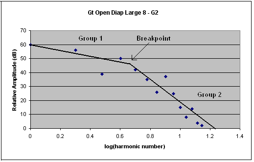
Figure 1. Spectrum of a Large Open Diapason pipe (tenor G). Two trendlines are also shown.
The blue dots in Figure 1 show the harmonic amplitude spectrum of the tenor G pipe (the G below middle C) from a 'large' open diapason rank which followed a sixteenth-note diameter halving progression. The scatter among the points is typical of that observed with organ pipe spectra, and it is largely due to the effect of standing waves within the building which affect each harmonic differently. The scatter-pattern also changes with listening position, thus if the recording microphone had been moved a completely different pattern would have been captured, yet the ear would still have been able to decide that the sound was that of an open diapason. It is this remarkable fact that first requires investigation. Observe that the pattern of harmonics falls naturally into two regions labelled Group 1 and Group 2 which have been approximated by the two trendlines drawn on the graph. The two lines intersect at a point which is called the 'breakpoint' here. It is noteworthy that this two-group structure is common to virtually all of the spectra I have examined over some forty years of research, embracing flute, diapason, string and reed pipes.
The justification for using a trendline approximation to represent a spectrum is that no two pipes of any organ stop sound exactly the same in terms of their timbres, even adjacent ones, and moreover the sound of any one pipe varies significantly at different points in the building as mentioned previously. Therefore there is no such thing as 'the sound' of an organ pipe in practice in the sense of it being unique or invariant. It is this intrinsic variability which enables trendlines to capture the essentials of spectra which are subject to these perturbations, because the lines themselves are not influenced as strongly as are the individual harmonics by random variations. They tend to 'iron out' the scatter among the harmonics. An important feature of trendlines is that they enable a spectrum to be represented using only three numbers in this case, namely the breakpoint or harmonic number at which the two lines intersect and the slopes of each line measured in decibels per octave. Thus the spectrum in Figure 1 is characterised by a number triplet with the values 4.5 for the breakpoint expressed in terms of harmonic number, -6 dB/8ve for the slope of the Group 1 trendline and -23 dB/8ve for the Group 2 slope. This is very much less than the 28 numbers which would otherwise have been required (the amplitudes and frequencies of 14 harmonics) and therefore it is much easier to handle. An expanded discussion of trendlines applied to organ pipe simulation and synthetic sample synthesis appears in another article on this site [5].
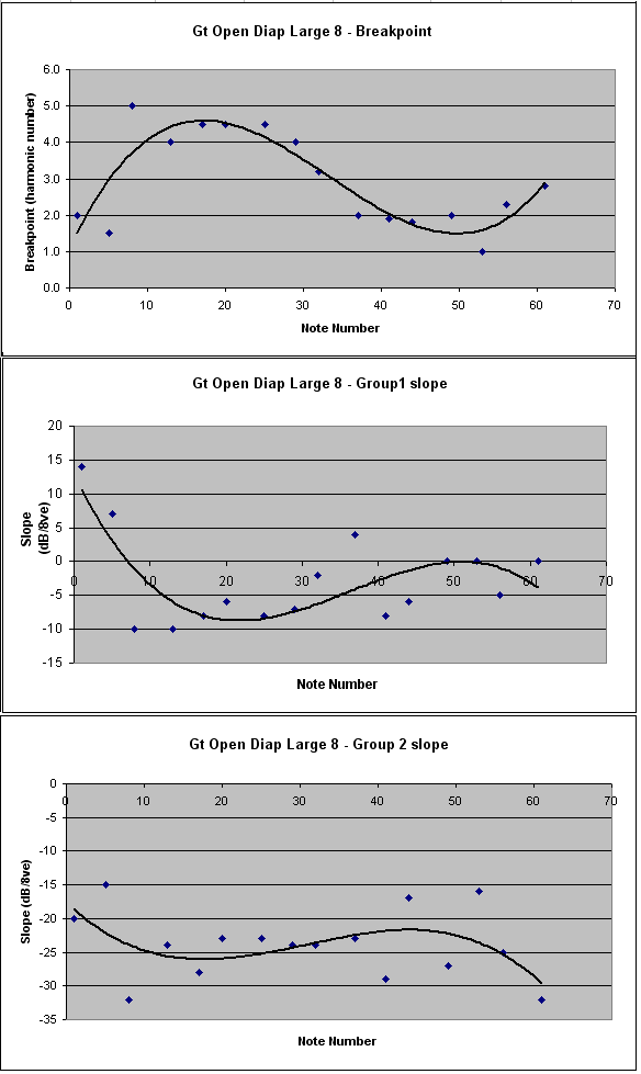
Next, we require the spectrum, now represented economically in trendline form, to be related to pipe scale. This was done as follows. The spectra of sixteen pipes equally spaced across this diapason rank (three per octave plus the top note) were computed and trendlines derived for each one. In each case the three numerical values defining the two lines were measured and then plotted in terms of their position in the key compass. This resulted in the three graphs shown in Figure 2, one for each trendline parameter. The horizontal axis of each graph represents note number running from 1 (bottom C) to 61 (top C).
Figure 2. Large Open Diapason - variation of trendline parameters across the key compass
The sixteen individual values of each trendline parameter (the breakpoint and the two line slopes) are represented by the blue dots in the respective graph. As with the individual spectra themselves there is quite a lot of scatter in evidence. However fitting curves to the graphs (the black lines) enabled some interesting behaviour to be identified. Firstly consider the slopes of the Group 2 trendlines as plotted in the bottom graph. These lines are those associated with the high order/low amplitude harmonics in each spectrum as shown earlier in Figure 1, and the slopes do not vary greatly across much of the compass despite the outlying points at each end. The mean value is about -24 dB/8ve which accords with what the eye can detect across the central region of the compass. It is possible that the changes in trendline slope towards the bass and treble, suggested by the black curve, are simply artefacts due to the random scatter in the data in these regions rather than indicating systematic behaviour. However such behaviour is nevertheless sensible because it suggests that more harmonics will be emitted by the bass pipes because the line slope becomes less steep than in the treble, where the reverse will apply. This is precisely the behaviour encouraged by a scaling law such as that used for this stop, which makes the bass pipes narrower relative to their speaking length compared with pipes in middle of the compass. Narrower pipes emit more harmonics, other factors being equal. Towards the treble the scaling law makes the pipes wider, thus they emit fewer harmonics, a feature also suggested by the graph. It is therefore possible that this graph is indeed reflecting spectral, and thus tonal, characteristics across the key compass which are related to the sixteenth-note scaling progression applied to this pipe rank.
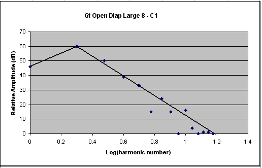
The other two parameters, the breakpoint and the slope of the Group 1 trendline, show an interesting feature towards the bass end of the compass. The breakpoint value decreases markedly, whereas simultaneously the Group 1 slope changes rapidly from a negative value to a positive one. Taken together, these result in significant changes in the spectra towards the bass. Higher in the compass a typical spectrum was shown in Figure 1, whereas in the bottom octave it becomes quite different. To illustrate this, the spectrum for the bottom note is shown in Figure 3 below.
Figure 3. Spectrum of a Large Open Diapason pipe (bottom C). Two trendlines are also shown.
Note how the Group 1 trendline now has a positive (upwards) slope whereas formerly it was negative. The breakpoint has also reduced markedly from its former value to lie at the second harmonic. These changes result in the pipe emitting a second harmonic of considerably higher relative amplitude than those further up the keyboard, and this effect also applies to some of the subsequent harmonics. For this pipe the second harmonic has reached five times the amplitude of the fundamental (14 dB), and even the third harmonic is about 1.6 times stronger (4 dB). This is quite different to pipes higher up the compass whose spectra are typified by that shown in Figure 1, where the strongest harmonic is the fundamental itself. This behaviour results in the bass pipes of this diapason stop sounding brighter and less ponderous than they would otherwise have done had no scaling been applied. This is partly a consequence of the relative narrowing of the pipes towards the bass conferred by a sixteenth-note halving interval. Therefore, again the data here are probably reflecting certain tonal characteristics which are related to the scaling of this rank.
To summarise, the curves in Figure 2 show how the spectra and thus the tone quality of this diapason stop vary across the key compass. This was only made possible through the use of three trendline parameters to represent the essentials of each spectrum, because it would otherwise have been impractical to reach any conclusions at all. It was further shown that some aspects of the curves are clearly compatible with the scaling law applied to the pipe rank. Perhaps the most important outcome is that we now have a concise set of templates, three in all, which jointly describe how the spectrum of a typical diapason stop varies across the compass. Similar sets of curves can also be derived in like manner for other classes of organ tone (flutes, strings and reeds), and for other musical instruments.
In practice some useful generic features of the templates can be extracted from qualitative observations on the graphs, and for diapasons the obvious simplifications are:
Group 1 slope Negative (slopes downwards) over most if not all of the compass. Gets steeper towards the bass (thereby preventing excessive development of the early strong harmonics which would make the sound too thin and stringy) and less steep towards the treble (which maintains the subjective loudness of the smaller pipes by distributing the power among more harmonics). However, and optionally, the second harmonic can be selectively emphasised in the extreme bass by changing the slope so it becomes positive (upwards gradient) as in Figure 2. If this is done a corresponding reduction should also be made to the breakpoint to prevent over-emphasising harmonics beyond the second (see below).
Group 2 slope Always negative (slopes downwards) over the compass. Value remains approximately constant over most if not all of the compass, but optionally it can become less steep in the bass (encourages development of the weaker higher-order harmonics and hence brightness) and/or steeper in the treble (reduces higher-order harmonic development, where they go beyond the range of audibility in any case).
Breakpoint Increases towards the bass (encourages development of a few strong early harmonics, thereby improving definition and reducing woolliness) and decreases towards the treble (reduces early harmonic development to prevent screaming). However, if the Group 1 slope swings positive in the extreme bass (see above), the breakpoint should simultaneously reduce to prevent over-emphasis of harmonics beyond the second. This behaviour can be seen in Figure 2.
Therefore if you only have the spectrum of a single diapason pipe, taken from the middle of the keyboard say, these results suggest how to scale other spectra upwards towards the treble and downwards towards the bass to represent a complete and consistently-scaled diapason rank. These conclusions and the means of deriving them are believed to be original.
Generating the synthetic samples
We can now go further and synthesise the corresponding waveforms for each note of a diapason rank from the set of scaled spectra. As just mentioned, the three graphs in Figure 2 contain enough information to reconstitute the spectra for an open diapason across the entire key compass. This follows because the three trendline parameters, the breakpoint and the two trendline slopes, can be extracted for each of the 61 notes. Using the method of Trendline Synthesis described in reference [5], a complete set of 61 synthetic samples can therefore be derived. A brief outline of Trendline Synthesis is given below for completeness.
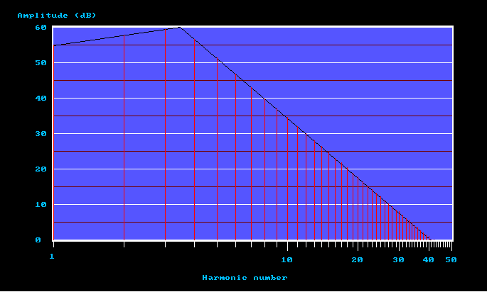
Figure 4. A typical trendline plot
Figure 4 shows a spectrum with two trendlines in which the harmonics are indicated by the red lines, though the diagram does not correspond to any particular organ tone as it is shown here purely for illustrative purposes. The first line has an upwards (positive) slope of 3 dB/8ve and the second has a downwards (negative) slope of -17 dB/8ve. The breakpoint is at a 'harmonic number' of 3.5. The quote marks serve to show that this is, in a sense, a fictitious number because it does not correspond to an actual harmonic, lying as it does between harmonics three and four, but it is more flexible for the breakpoint not to be restricted to integer values. There are 42 harmonics enclosed by the two trendlines. This type of graph is the most important output screen of an interactive design program which I have developed (written in C). Note that the number of harmonics is not required of the user, as this parameter drops out of the process automatically as a consequence of merely having defined the two trendlines.
What does one do with this picture? As stated already, it is only necessary for the user to specify the slopes of the two lines and their breakpoint, that is, to input just three numbers. The screen then appears and harmonics are drawn in automatically as shown by the red lines in the diagram. Their amplitude values are used to generate a Windows wave file by additive synthesis (a standard PCM file with a WAV extension) which can then be auditioned in a sound sampler or wave editor. To facilitate this, loop points are created automatically and embedded in the WAV files so that the sound lasts for as long as the user wishes. The same looped WAV file can also be imported into one of many external rendering engines such as a software synthesiser or an existing digital organ system, when other articulation parameters such as attack and release envelopes will be added to complete the voicing of the sample.
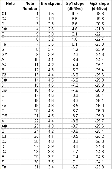
Extracting the three trendline parameters for each note of the diapason rank we have been discussing can be done in principle simply by measuring their values from the graphs in Figure 2, though in practice this is an impossibly laborious task. A much simpler method is to use the equations of the three black curves in Figure 2. These equations are available because the curves were fitted mathematically to the corresponding data points using an Excel spreadsheet, and if you ask Excel to fit a curve it also gives you the equation of the curve it comes up with. Therefore we can easily generate in the same spreadsheet a complete set of trendline parameters for each note across the keyboard, and from these parameters as many synthetic diapason samples as desired can be computed using Trendline Synthesis as above. Some of the trendline parameters, representing the black curves in Figure 2, are shown in the table below (Figure 5).
Figure 5. Some of the trendline parameter scaling values corresponding to the curves in Figure 2.
Figure 5 is an extract from the complete table, showing the three trendline parameters for each note covering the lower half of the keyboard. Thus for each note a corresponding synthetic waveform can be synthesised as outlined above, the important point being that the complete set of 61 samples so obtained is scaled convincingly across the key compass. However, as pointed out in the previous section, the trendline data can be simplified if desired by reducing them to a more qualitative generic form which might find wider applicability.
It will not have escaped the notice of the reader that there is considerable scope for automation here (using batch processing) in the production of a complete synthetic sample set. This makes the technique attractive when compared with the expensive tedium of creating samples using recordings of organ pipe sounds, even in those cases where it is possible.
An interesting and useful aspect of the data table shown in Figure 5 is that it can be used to derive ranks at pitches (footages) other than the unison (8 foot) rank which was analysed originally. This is possible because the values in the table are equivalent to the scaling charts used by organ builders for ranks of organ pipes. Therefore parameters can be derived for any desired pitch, thereby offering the possibility of generating a complete diapason chorus in which each rank is scaled properly yet independently relative to the others.
To illustrate this, consider a 4 foot diapason or principal rank. In a pipe organ this would normally consist of pipes with slightly different diameters, pitch for pitch, compared with the unison rank. Thus the bottom C pipe on the 4 foot rank would be slightly different than tenor C on the 8 foot one, even though their pitches would be nominally identical. This results in slightly different tone qualities between the two ranks, thereby enhancing the aural interest of a chorus of stops as well as assisting blend. Typically the 4 foot rank would be scaled two or three semitones smaller in terms of pipe diameter than the 8 foot one. Exactly the same thing can be done using the table above when generating synthetic samples. Bottom C on a 4 foot rank might use the parameters corresponding to notes D2 or D#2 rather than C2, whereas it would be tuned to the same frequency as C2. Note that this is not the same thing as deriving the 4 foot rank from the 8 foot one by extension from a single rank. By definition, extension organs cannot be scaled independently at all pitches, which is one of their several disadvantages.
Similarly, ranks at other pitches can be scaled in like manner. A 2 foot stop, mutations and mixtures can all be generated in the same way by picking off the trendline parameters from the scaling chart, though they would usually start a few notes smaller still than the 4 foot rank just discussed. They might also use a slightly different, usually slower, diameter-halving interval. This illustrates the flexibility of this method of creating a synthetic sample set which is nevertheless based entirely on data derived from the sounds of real instruments.
The audio clip below is of two synthetic Open Diapason stops, one 'large' and the other 'small', used together to play the hymn tune 'Westminster Abbey'. Both are of 8 foot pitch. The 'large' diapason was synthesised using the scaling values shown in Figure 5, whereas the 'small' one started three notes smaller in the bass (i.e. it used the trendline parameters listed for D# to generate its bottom note). At the keyboard the characteristically warm and spacious sound one would expect when using the two equivalent ranks on a pipe organ is wholly convincing.
When simulating musical instruments using synthetic samples it is necessary to scale the samples across the key compass to imitate the variations in timbre or tone quality which occur in the real acoustic instruments. In the pipe organ, each pipe comprising an organ stop is scaled (dimensioned) deliberately to encourage its timbre and loudness to remain subjectively of a piece across the rank. For example, cylindrical pipes of diapason (principal) tone quality are often scaled so that their diameters halve at the interval of a major tenth, in contrast to their speaking lengths which perforce must halve every octave.
This article has shown how this type of scaling law affects the harmonic spectra of the pipes by representing each spectrum by two trendlines. Only three numbers are required to define the trendlines, namely their point of intersection and their slopes, which is considerably fewer than attempting to specify a spectrum using the amplitudes of its constituent harmonics. An additional reason for using a trendline approximation to represent a spectrum is that no two pipes of any organ stop sound exactly the same in terms of their timbres, and moreover the sound of any one pipe varies significantly at different points in the building. This intrinsic variability enables trendlines to capture the essentials of spectra which are subject to these perturbations, because the lines themselves are not influenced as strongly as are the individual harmonics by random variations - the lines tend to 'iron out' the scatter among the harmonics.
Variations in each of the three trendline parameters for a real diapason stop across the key compass were presented and explained in terms of its scaling. The results suggest how to scale the spectra of a synthetic sample set upwards towards the treble and downwards towards the bass to represent a complete and consistently-scaled diapason rank, and it was shown how wave samples can be derived from the trendline parameters for use in a sound sampler. It was also shown how the data can be used to generate similar sample sets for diapason stops at different pitches which are properly scaled in relation to the unison rank, just as in a pipe organ.
The method of sound creation described here stands midway between sampled sound synthesis on the one hand and physical modelling on the other. Sampling real acoustic instruments can provide a convincing re-creation of the instrument which was sampled, but the result is inherently inflexible because it is difficult to make other than minor adjustments to the sample set. Physical modelling stands at the opposite pole. It provides a degree of flexibility limited only by the capabilities of the models used, but the outcome does not necessarily bear any relation to the sounds of the instrument being modelled because these play no part in generating the waveforms. Thus the results veer towards the generic rather than the specific. Synthesising sounds synthetically using the approach illustrated here is based entirely on data derived originally from the sounds of real instruments, yet the data can be manipulated easily to yield a high degree of voicing flexibility in the end result.
The method is general and it can therefore be applied when simulating the other classes of organ tone (flutes, strings and reeds) as well as other musical instruments.
1. "Re-creating Vanished Organs", an article on this website, C E Pykett, 2005.
2. "The physical modelling of organ flue pipes - a complete picture", an article on this website, C E Pykett, 2013.
3. "How the flue pipe speaks", an article on this website, C E Pykett, 2001.
4. "The End Corrections, Natural Frequencies, Tone Colour and Physical Modelling of Organ Flue Pipes", an article on this website, C E Pykett 2013.
5. "Trendline Synthesis - a new music synthesis technique", an article on this website, C E Pykett 2016.
|