A technique for simplifying parameter estimation in synthesised organ pipe sounds
Colin Pykett
Posted:
15 November 2017
Revised: 23 October 2024
Copyright © C E Pykett
Abstract. A major problem in synthesising musical sounds lies in assigning values to the large number of parameters associated with each note. For example, in additive synthesis the relative amplitudes of each harmonic have to be specified together with the way each one varies throughout the sounding epoch. Or in a physical model of an organ flue pipe the parameter set describing the aerodynamics of the pipe foot and mouth, as well as the properties of the resonant air column, likewise becomes inconveniently large. In such cases allocating values to the parameters to achieve a desired timbre is therefore a major challenge. The problem is particularly difficult for the organ because each stop is in effect a different instrument with a distinct character. Furthermore each stop also comprises many separate notes which all have to be individually voiced. This results in a serious parameter overload and estimation problem in current synthesis techniques for simulating the pipe organ.
This article describes a method which requires only four parameters to define the steady-state timbre of any organ pipe. This is very much smaller than the parameter lists used in traditional tone models whose sizes might run to fifty or more. Furthermore the parameters are intuitive rather than arcane descriptors of sounds, thus it is unnecessary for a voicer or tonal designer to be a specialist in digital music.
A complete digital organ simulated in this manner is described together with sound files demonstrating the wide range of sounds it can produce.
Contents
(click on the headings below to access the desired section)
Introduction
Simulating the pipe organ - the importance of the sustain phase
Simulating organ pipe sounds using only four parameters
A complete instrument
Concluding remarks
Notes and references
Introduction
There are basically two ways to synthesise musical sounds. Either samples are recorded from a real acoustic instrument or they are created synthetically using one of several techniques. The first method is widely used though it is not really synthesis as such because the target sounds already exist, being merely recorded and then played back under computer control. It has the advantage that the sound of a particular instrument at a particular listening position in a particular room can be reproduced very closely. However this very particularity means that it is an inherently inflexible technique in that the possibilities for voicing are limited. Only simple changes can be made such as tuning a sample, varying its volume or applying EQ. Making a more subtle change, such as adjusting the cut-up of a simulated organ pipe, is impossible because then you are moving away from real sounds towards synthetic sample creation. On the other hand, a sample generated synthetically from the outset can be adjusted as required as part of the process of producing it. It is your own created entity and in principle there are few limits on what can be achieved.
Synthetic samples can be constructed in two ways - signal modelling or physical modelling. The first includes a raft of techniques going back to the earliest days of electronic music, including additive, subtractive or FM synthesis. The second, physical modelling, models the acoustic architecture of the real instrument rather than the sound waveforms which it emits. However both approaches suffer from the same dilemma in that the almost unbounded flexibility they offer is both an advantage and a hindrance. Modelling of either kind is attractive in view of the many options available for creativity, yet simultaneously difficult because of the many parameters involved in generating the sounds. As an example, additive synthesis can reproduce exactly any desired sound in theory, but in practice it requires the amplitudes of many harmonics to be specified together with the way each changes over the sounding epoch. Physical modelling likewise demands that numbers be allocated to a wide range of parameters describing the instrument being modelled, but many of them can only be approximate or even just guesses. In both cases the parameter list for generating a single note is formidable - it can run to several tens if not hundreds of entries and all of them have to be assigned largely by hand and often by trial and error at the present state of the art. Consequently pressure continues to build up within the digital music community to solve the parameter overload and estimation problems (see reference
[1] for an example relating to Viscount's physically-modelled 'Physis' organs). What are needed are far fewer parameters, together with interactive and slick means for assigning values to them. In other words, voicing tools are required which should be useable at an intuitive level by those with 'golden ears' who will often not be specialists in computer-generated sound. This article describes a synthesis technique which requires only four parameters to define almost any conceivable organ pipe timbre.
Simulating the pipe organ - the importance of the sustain phase
As with other instruments, synthesising pipe organ sounds is afflicted by the generic problem of assigning values to a large number of parameters as outlined above. It might be thought that one way to do it would be for the tonal designer to sit down with an experienced pipe organ voicer and use the ears of the latter to arrive at a suitable parameter set. This is indeed sometimes done, though it is expensive and time consuming and there still remains an element of hit-and-miss in the results achieved. One reason for this is that the parameters presented to the voicer are often not those s/he can naturally identify with - someone who usually deals with things like cut-ups and nicking is unlikely to feel immediately at home with a nonlinear digital filter forming part of the jet-drive model of a flue pipe. Nevertheless, an organ pipe is one of the easiest 'instruments' to simulate for one simple reason in that its subjective timbre is dominated by the spectral structure, the harmonic recipe if you will, of its sound during its steady state (sustain) phase. Other instruments do not have the advantage (from a synthesis viewpoint) of such a stable sustain phase whose duration is arbitrarily long. To be sure, several other parameters are also important such as the attack transient, small random variations in frequency and amplitude, and aerodynamic noise. However in moderate-sized or larger rooms and at realistic listening distances these other factors become less important to a listener than the sustained sound of a pipe. This premise is no doubt arguable, but it remains a fact that if you cannot simulate the steady state sound of an organ pipe adequately then the simulation will also be unsatisfactory, by definition. The simulation will not sound like an organ at all.
Proceeding on this basis, it is therefore necessary to assemble a range of computer-based tools which will simulate the sustained sound of any organ pipe in a simple and intuitive manner. In particular, the toolset must be interactive, one which an organ voicer can rapidly become familiar with, and which s/he can use to come close to the desired timbre in a matter of seconds rather than minutes or hours. This is essential if the tools are to mirror the speed and facility with which a skilled crafts-person can voice a real pipe. Once having achieved the desired steady state timbre, the other articulation parameters mentioned above can then be added subsequently. But the point is that you cannot do the latter until you have first accomplished the former.
The simulation methodology in this article follows a signal modelling paradigm rather than using physical modelling because this choice enables the desired timbres to be attained more directly and easily. It is further assumed that a time domain sample for each simulated pipe is generated using the techniques to be described, so that a complete set of synthetic samples can subsequently be imported into one of the wide range of samplers and commercial digital organs now available.
Simulating organ pipe sounds using only four parameters
A technique has been developed which requires only four parameters to simulate accurately virtually any organ tone colour across the traditional tonal classes of flutes, diapasons, strings and reeds. In fact only three parameters are necessary in most cases. With such a small parameter set and the appropriate interactive software tools it therefore becomes a straightforward and rapid task to voice the sounds to one's satisfaction. The parameters are also relatively intuitive and easy to understand even by those whose skills lie elsewhere than in digital music. Thus musicians and pipe organ voicers should experience little difficulty in coming to grips with the processes involved.
As a case study we shall first look at the frequency spectrum of a Trumpet pipe speaking middle C as shown in Figure 1.
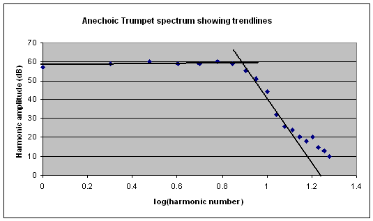
Figure 1. Harmonic structure of a Trumpet pipe speaking in anechoic conditions
The pipe sound was captured in an anechoic environment, thus its spectrum was not distorted by room effects such as standing waves (modes), phase interference due to multipath propagation and frequency-dependent damping caused by soft furnishings and carpets. The amplitudes of the harmonics are denoted by the blue dots. Note the smoothness of the spectral envelope. This is an important feature not usually seen in spectra derived from pipes speaking in ordinary rooms, and we shall return to it later.
Superimposed on the spectrum are two linear trendlines, approximating respectively to the flat envelope associated with the first seven harmonics and the steeply-descending envelope of the remainder. These harmonic groups are denoted as Group 1 and Group 2 respectively in this article. The lines intersect at a point lying between the seventh and eighth harmonics. A beguiling question therefore arises. Because it is apparently so easy to approximate closely to the real spectrum using only two straight lines, might it be possible to use them to represent the spectrum rather than using all the constituent harmonics? And how accurately would this approximate spectrum recreate the original sound of the real organ pipe? The advantage of using just the two lines is that only three parameters are necessary to define them, namely their slopes and their point of intersection. Compared with the nineteen harmonic amplitudes in the original spectrum that would otherwise be required, this represents a very considerable simplification of the parameter estimation problem. To answer these questions, consider the same Trumpet spectrum but now regenerated from the two trendlines as shown in Figure 2.
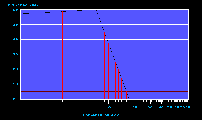
Figure 2. Regenerated Trumpet pipe spectrum using two linear trendlines
The two trendlines are shown as before, and a retinue of harmonics has been plotted as the red lines. But all the harmonic amplitudes are now defined solely by the trendlines - the harmonics no longer have a direct connection with the original Trumpet pipe sound as they did in Figure 1. It is now solely the two lines which have captured the flavour of the original sound, and they impose this in the form of a spectral envelope on the harmonics. It can be seen that the main features present in the original spectrum have been largely retained, including the numbers of harmonics in the two cases (19 harmonics originally; 17 in this reconstruction)
[4]. The three parameters defining the trendlines are:
Breakpoint (point of intersection) at a harmonic number of 7.25
Slope of Group 1 trendline (representing the first seven harmonics) : + 1 dB/octave
Slope of Group 2 trendline (representing the remaining harmonics) : - 48 dB/octave
Applying additive synthesis to the two spectra demonstrates that the sound of the original Trumpet pipe and that produced by the trendline spectrum are virtually identical, and the audio file below confirms this. The first sample on the recording corresponds to the real Trumpet followed by the version regenerated using the trendlines. Each sample is about ten seconds in duration separated by a gap lasting a few seconds:
 Demonstration of real and regenerated Trumpet pipe sounds - 484 KB/30s
Through detailed research undertaken over the last two years (2015 to 2017) it has been found that only two trendlines are required to define almost any conceivable organ pipe spectrum. Thus the wide range of conventional organ timbres, ranging from liquid flutes, through robust diapasons, keen strings and assertive reeds can all be synthesised in a similar way. Some further audio examples are given later to prove the point. Many organ tone colours can be simulated accurately by assigning values only to the three trendline parameters described above, namely the breakpoint and the two line slopes. However some tones require a fourth parameter, a single number which controls the relative amplitudes of the even and odd harmonics in the spectrum. Examples of pipe tones where this is necessary are most flutes, and reeds such as the Clarinet and Vox Humana. Deriving the parameter set for a given tone, or voicing a simulated pipe in other words, can be approached in two ways. Initial estimates can be obtained quickly if the frequency spectrum of a prototype pipe is available, and this was illustrated above in Figure 1. The estimates can then be refined by ear if desired using suitable interactive voicing tools. Or the initial estimates can simply be 'invented' once sufficient experience has been gained, again followed by voicing to taste. Both methods have their place in voicing a complete organ stop, where it is possible to derive the entire parameter set across the compass having used only a single prototype pipe spectrum in the middle of the keyboard as a guide.
It might be argued that the smooth spectrum envelopes generated by trendline synthesis are unrealistic and that they will lead to tones which lack aural interest. However some recordings are available below and they do not really support this criticism. Moreover Figure 1 confirms that real organ pipes also generate similarly smooth spectra, though examples are rarely seen because of the difficulty and expense of recording pipes anechoically. It is largely room effects which are responsible for distorting a pipe's harmonic structure by imposing the amplitude scatter which is usually observed when spectra from in-room recordings are examined. As mentioned above, these effects include room modes, phase interference and damping. Because such ragged spectra are so ubiquitous this seems to have led to a view that the initial radiated spectrum from the pipe is also of this form. The results here have demonstrated that this is not so.
It is also the case that room effects are strongly spatially-dependent over short distances as demonstrated in Figure 3.
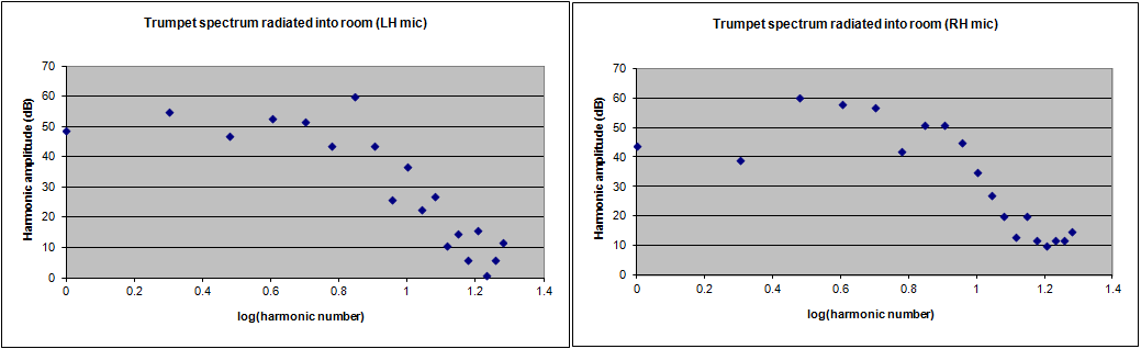
Figure 3. Radiated Trumpet spectra received by two microphones 13 cm apart.
These plots were obtained by replaying the anechoically-derived Trumpet tone (spectrum in Figure 1) into an ordinary (non-anechoic) room using a high quality loudspeaker. Signals were picked up on a matched stereo pair of studio microphones 13 cm apart, and their spectra are shown in the diagram. Not only was the room responsible for the observed scatter, but also for the gross differences in spectrum shape occurring over this short distance. Unsurprisingly, the signals from the left and right channels sound appreciably different, and in general such room disparities swamp the minor differences that might arise between the sound of a real pipe and its trendline approximation. It is when one sees results such as this that one begins to realise why trendlines work so well in capturing complex sounds - presumably the lines average out the random amplitude scatter and enable the essentials of the sound to survive the spectral distortions due to room ambience. It is therefore unnecessary to impose artificial scatter on the smoothly-varying harmonic amplitudes arising from this type of synthesis because any real room will do the job for you, just as it does for the sounds of actual organ pipes.
Other articles elsewhere on this site discuss synthesis using trendlines in more detail. Reference
[2] is an overview of the subject. Reference
[3] examines the problem of scaling, or how to vary trendline parameters across the compass to simulate the scaling of real organ pipes.
A complete instrument
Creating individual notes with desirable timbres can only take you so far. Beyond that it is necessary to construct a complete organ stop comprising many properly-scaled notes across the entire key compass, and then go still further by incorporating several such stops into a complete and playable instrument. Only then can a synthesis technique be fully evaluated in a musical sense, such as how each stop blends and combines with the others. This is a non-trivial undertaking because hundreds of tones have to be voiced to produce a unique set of parameters for each one. Even when only three or four parameters for each sustained tone have to be adjusted, as here, it still involves a lot of work. The magnitude of the task when there might be more than fifty does not bear thinking about, hence the importance of reducing the parameter overload problem - which is what this article is all about. In this case a demonstration organ with two manuals and pedals was created with the disposition shown below. It is romantic rather than classically voiced, and although relatively
small there is plenty of colour available and it can also pack a punch when necessary.
PEDAL |
|
SWELL |
|
GREAT |
|
| Violone |
16 |
Geigen Diapason |
8 |
Open Diapason |
8 |
| Bourdon |
16 |
Chimney Flute |
8 |
Claribel Flute |
8 |
| Principal |
8 |
Geigen Principal |
4 |
Dulciana |
8 |
| Bass Flute |
8 |
Stopped Flute |
4 |
Principal |
4 |
| Trombone |
16 |
Mixture 15.19.22 |
III |
Fifteenth |
2 |
| Trumpet |
4 |
Double Trumpet |
16 |
Trumpet |
8 |
|
|
Cornopean |
8 |
|
|
| Great to Pedal |
|
Clarinet |
8 |
Swell to Great |
|
| Swell to Pedal |
|
Clarion |
4 |
|
|
|
|
|
|
|
|
|
|
Tremulant |
|
|
|
The instrument physically exists in that it can be played in real time in the usual manner, and sound generation uses the Prog Organ digital platform
[5]. This is a sound sampler optimised for organ applications, therefore each note of each stop has to be associated with a wave sample generated in this case from a group of trendline parameters. Thus a substantial sample set had to be synthesised before importing it into the system, and the following audio examples demonstrate something of the results. The Prog Organ synthesisers were programmed to impose a small amount of random frequency movement on the samples to simulate wind pressure fluctuations in a pipe organ, and this can sometimes be heard on sustained notes. All recordings are in stereo.
(a) The Claribel Flute. These liquid tones use a parameter set derived from studying spectra of a stop of this name on the Rushworth and Dreaper organ at Malvern Priory, England.
'Moderato' (W G Alcock) - 940 KB/1m
(b) 'Large' and 'small' unison diapason stops played together (the small diapason does not actually appear as a manual stop in the version of the stop list shown above, where it is only used as the pedal organ Principal. However the large diapason is the Open Diapason on the great. Thus the recording was made using a slightly different disposition.)
Hymn tune 'Westminster Abbey' (H Purcell) - 787 KB/50s
(c) Demonstrations of some other stops - here another hymn tune (Wareham) is played successively on the swell 8 and 4 foot Flutes, a Clarinet solo, a Cornopean solo, a Trumpet solo and finally full organ (save the Trumpet). The swell flutes simulate heavily-nicked romantic pipework in that their attack transients are more or less suppressed. The Clarinet is modelled on the sounds of a Wurlitzer specimen, one of the finest pipe organ clarinets I have ever come across especially in the tenor register. The Cornopean is midway in tone and power between an Oboe and a Trumpet. Its 16 and 4 foot siblings in the swell reed chorus also have a similar tone. The great Trumpet is conceived as a solo rather than a chorus reed, being loud, brassy and assertive. It is rather like the high pressure Military or Fanfare Trumpet stops found in large pipe organs, and it 'comes on with a crack'.
Hymn tune 'Wareham' (W. Knapp) - 2.29 MB/2m 30s
(d)
Another piece from Walter Alcock in quiet and reflective mood. It was
written in memory of C H H Parry and has no title.
'Rather slowly' (W G Alcock)
- 1.77 MB/1m 56s
I have not assumed that you will necessarily like these sounds as that is not the point of this article. They are included mainly to demonstrate the wide range of timbres which can be created using this technique. Requiring only four parameters, its simplicity enables you to rapidly voice a synthesised tone to meet your own preferences once you have gained some familiarity with it.
In practice, using a sound sampler such as Prog Organ is probably not the optimum method of rendering sounds created in this manner. The two stage process used here, of first synthesising a set of sample waveforms and then importing it into a sampler, could be streamlined if a customised rendering engine was used which could accept the trendline parameters for each note directly. This would not be overly difficult to implement using off-the-shelf DSP chips. Interactive voicing and tonal finishing operations could then take place within the instrument itself.
Concluding remarks
A major problem in synthesising musical sounds lies in assigning values to the large number of parameters associated with each note. For example, in additive synthesis the relative amplitudes of each harmonic have to be specified together with the way each one varies throughout the sounding epoch. Or in a physical model of an organ flue pipe the parameter set describing the aerodynamics of the pipe foot and mouth, as well as the properties of the resonant air column, likewise becomes inconveniently large. In such cases allocating values to the parameters to achieve a desired timbre is therefore a major challenge. The problem is particularly difficult for the organ because each stop is in effect a different instrument with a distinct character. Furthermore each stop also comprises many separate notes which all have to be individually voiced. This results in a serious parameter overload and estimation problem in current synthesis techniques for simulating the pipe organ.
This article has described a method which requires only four parameters to define the steady-state timbre of any organ pipe. This is very much smaller than the parameter lists used in traditional tone models whose sizes might run to fifty or more. Furthermore the parameters are intuitive rather than arcane descriptors of sounds, thus it is unnecessary for a voicer or tonal designer to be a specialist in digital music.
A complete digital organ simulated in this manner was described together with sound files demonstrating the wide range of sounds it can produce.
Notes and references
1. "Introducing Deep Machine Learning for Parameter Estimation in Physical Modelling", C Zinato et al, Proc. 20th Conference on Digital Audio Effects, Edinburgh UK, September 2017.
This paper began by saying that "one of the most challenging tasks in physically-informed sound synthesis is the estimation of model parameters to produce a desired timbre". It disclosed that Viscount's physically-modelled 'Physis' organs use 58 "macro-parameters" for each simulated pipe, "some of which are intertwined in a non linear fashion and are acoustic-wise non-orthogonal (i.e. jointly affect some acoustic feature of the resulting tone)". That the paper appeared a decade after the introduction of these instruments demonstrated
the continuing importance of solving the parameter overload and estimation problems in physical modelling.
A
subsequent paper took the approach further:
"A
Multi-Stage Algorithm for Acoustic Physical Model Parameters Estimation", C
Zinato et al, IEEE/ACM Transactions on Audio, Speech, and Language Processing,
27(8), August 2019.
It
concluded that "preparing a complete stop required an effort that is of the
order of magnitude of a working day (8 hours) split in several sessions to
recover from fatigue, while with the proposed approach and the current
computational resources one stop can be prepared in approximately 5 minutes to
which some human effort must be added to judge on the result and conduct some
final adjustments"
It
is unclear from the paper whether this has since been achieved or whether it
remains a statement of intent. However no criticism of Viscount's products
is implied, since the firm is merely reflecting the difficulty of the parameter
estimation problem in the physical modelling approach to synthesising the sounds
of acoustic musical instruments.
2. "Trendline Synthesis - a new music synthesis
technique", an article on this website, C E Pykett 2016.
3. "Scaling synthetic samples across the key
compass", an article on this website, C E Pykett 2016.
4. The trendlines in Figures 1 and 2 are not quite identical because those in Figure 2 have been adjusted slightly to obtain a better aural match to the original sound.
5. "Prog Organ - a Virtual Pipe Organ", an article on this website, C E Pykett