


|
|
|
Signals, Noise and Bit Depth in Virtual Pipe Organs by
Colin Pykett Posted: Last revised: Copyright
© C E Pykett 2012
"The first condition for making music is not to make a noise" José Bergamín
"The average voice is like 70% tone and 30% noise. My voice is 95% noise." Harvey Fierstein
Abstract.
This article discusses two issues which arise when preparing waveform sample sets
for virtual pipe organs: the recording bit depth and how to remove noise from them.
The dynamic range of organ pipes extends
from that with the greatest SPL to the weakest harmonic of that with the smallest. An example
is given of an
organ whose dynamic range lies within 16 bits but without much
of a safety margin. Therefore it is suggested that at least 20 bits would be a realistic working
minimum, though this could be reduced by judiciously varying the gain to match
the level of the sample being recorded. Noise on the samples is dominated by the organ
blower. Three ways of reducing it are high and low pass filtering to reduce outband
noise, conventional subtractive noise reduction, and the
application of VPO-specific tools. A
custom tracking comb filter is described which capitalises on the different power distributions of noise and
signal as a function of frequency - noise exists at all frequencies across a
significant part of the audio spectrum whereas the wanted signals have their
power confined to well defined harmonics. This
difference enables the amplitude and frequency of each harmonic or partial to be
tracked automatically from the start of the attack transient of the sound, through the sustain phase
and then to the end of the release transient including room ambience.
Because power at all other frequencies is ignored, the result is
completely noise free.
Contents (click
on the subject heading to access the desired section) Audio bit depth for recording organ pipe sounds Reducing noise on waveform samples in virtual pipe organs Outband noise reduction - high and low pass EQ Frequency
domain noise reduction A tracking comb filter optimised for virtual pipe organs
This article is aimed at those with a particular technical interest in
the virtual pipe organ (VPO) rather than digital organs more generally; this is
because of the more open culture of the VPO community compared to that of
commercial digital organs. Also
some of the latter are less technically capable of simulating certain aspects of
pipe sounds than are most VPOs. For
those who might not be familiar with the VPO my Prog Organ system
featured on this site is an example, and further information about the more
general scene is given here at reference [1].
The cost effectiveness of the VPO as a method of simulating the pipe
organ makes it worth addressing in this article, which covers a number of
technical issues. These have been
selected because they feature frequently in the correspondence I receive.
Two topics constantly recur: the issue of bit depth (how many bits should
be used when recording organ pipe sounds digitally to produce a waveform sample
set), and the major problem of noise reduction (because any residual noise on
the sampled waveforms, particularly that from the organ blower, will build up
unpleasantly as more notes are keyed simultaneously).
Both issues are particular aspects of the more general topic of signal to
noise optimisation. The standard techniques used for recording and noise reduction across
the digital audio industry are not always be applicable to the particular case
of virtual pipe organs. On the
contrary, the techniques used need to be chosen with this speciality in mind.
I have even found it necessary to invent techniques which appear to be
novel, and one of the most useful of these (an auto-tracking comb filter) will
be described later. This is because the signals we deal with in VPOs are quite
different to those usually encountered in digital audio more generally, and the
differences are advantageous. For
example, we seldom need to handle the entire audio bandwidth for every waveform
sample because its lowest frequency is always that of the fundamental (pitch)
frequency, which is more often than not well above the usual hi-fi low frequency
limit. At the opposite end of the
spectrum, the highest frequencies in many pipes do not approach the limit of
human hearing. Furthermore, the
signal power within each sample is concentrated in its harmonic frequencies
rather than at the frequencies between them, whereas the reverse applies to the
noise. These properties of VPO
waveform samples can be helpful in noise reduction.
All this contrasts with ‘ordinary’ digital audio which has to cater
for recording and reproducing, say, a symphony orchestra in which music power
can arise at any frequency across the entire audio spectrum at unpredictable
times. It is therefore not
surprising that the generic toolkit used for processing recorded signals in
digital audio is not necessarily optimal or sufficient for recording and
processing the sounds of individual organ pipes one at a time, the somewhat
geeky activity which is meat and drink to the VPO specialist.
And who am I to lay down the law in these matters?
Well, I am not going to do so. I
do not claim particular expertise beyond that of others in the field, though I
have probably been in it for longer than many.
I first ‘sampled’ a large pipe organ in 1979 when digital audio and
personal computers as we know them today hardly existed.
(And anyone interested in how difficult it was to carry out operations
which are much simpler nowadays can see how things had to be done then in
reference [3]). So to answer my own
question, I merely throw this
article into the pool of user experience with VPOs with the hope it might be of
some interest. Audio
bit depth for recording organ pipe sounds Bit depth signifies the number of bits used to encode each waveform
sample value when making digital recordings or when processing them afterwards
in a computer. At the risk of being
pedantic, we need to distinguish between the two different contexts of the word
‘sample’ used in this article. As
just used, it refers to the instantaneous digital value of an audio waveform as
it is repetitively measured or ‘sampled’ by an analogue to digital
converter. The other usage means an
entire waveform snippet, perhaps several seconds in duration, which is the
entity captured when ‘sampling’ a pipe organ to produce a ‘sample set’. An audio CD uses 16 bit samples; this standard is offered by many
digital recorders and it is still used widely.
However it is being superseded by greater bit depths, up to 24 in the
most expensive equipment. Mid-range
or older recorders might offer an intermediate value between these two figures.
On the basis of the correspondence I receive, it seems that some VPO
enthusiasts insist that 16 bit recording can never be satisfactory, whereas
others are not so sure and they maintain that 24 bits is over the top and not
cost-effective. To try and
illuminate the issues, if not resolve them, it is instructive to put some
numbers into the arguments. The
numbers here will ultimately relate to the specific VPO scenario rather than to
digital audio in general, but let us begin with some general issues first. In round figures each bit provides a dynamic range contribution of 6 dB
(a ratio of two in voltage), where dynamic range means the ratio between the
largest and smallest voltages which can be recorded. Therefore a 16 bit system offers 96 dB and a 24 bit one 144
dB. These compare with the dynamic
range of human hearing at about 140 dB, whereas that of a very good capacitor
(studio quality) microphone is limited to about 125 dB (equivalent to about 21
bits) by its associated analogue circuitry and the onset of excessive
distortion. Such a microphone
should be used for recording organ pipe sounds, and therefore on the face of it
a 21 bit digital recorder is implied if one wants to get the best out of a top
quality microphone. However it is
worth looking at the issues in more detail first. If the maximum voltage at the output of a digital recorder is assumed to
be 2.5 volts rms, a typical figure, then the use of 24 bits means that the
minimum resolvable voltage is a minute 160 nV rms approximately.
It is useful to compare this with the thermal noise from a resistor
because this sets a practical limit to the minimum voltages which can be used in
any analogue circuit – its theoretical minimum noise floor.
We have to consider analogue circuits because the microphone signals are
not digitised until they reach the recorder.
For example, a 1000 ohm resistor at room temperature generates a noise voltage of about 550 nV
rms (something over half a microvolt) in a bandwidth of 16 kHz, which spans the
frequency range of a young adult’s
hearing. This is much greater than
the above figure of 160 nV. For
practical engineering reasons, capacitor microphones necessarily must use an
integrated impedance matching circuit such as an emitter follower to match the
very high impedance of the capacitive transducer into the connecting cable and
its circuitry at the remote end. The
matching circuit will typically have an output impedance up to about 1000 ohms,
hence the choice of resistor value in the example above.
It will therefore define a system noise floor both from thermal noise in
its passive components and from noise in its transistors, to say nothing of
noise on the necessary DC supply delivered to the microphone down its cable,
which is a factor often overlooked. Therefore
it is unfeasible that the electronic noise voltage at the output of the
impedance matcher (i.e. at the microphone output) could be reduced below the 550
nV rms figure just mentioned, and in reality it will be greater.
This contributes to the 125 dB dynamic range limitation of capacitor
microphones mentioned above, and it far exceeds the minimum resolvable signal of
about 160 nV rms at the output of a typical 24 bit digital system. So where are we? In theory
24 bit recording exceeds the dynamic range of the ear by a few dB, and if
one’s ear was actually bombarded with the maximum signal implied by this
figure (well into the threshold of pain) it would thereafter cease to work
properly, if at all. But the
best microphones are limited to about 125 dB, 19 dB or about 3 bits below the
144 dB dynamic range of 24 bit sampling. This
means that the least significant 3 bits or so would merely be continually
encoding thermal and electronic noise from the microphone even under the most
benign conditions imaginable (i.e. with absolutely no acoustic signal being
picked up from the room). As rooms
cannot possibly be this quiet, this is unachievable and therefore one might be
forgiven for asking, as some people do, why 24 bits for live (microphone)
recording should be used at all. On
the face of it 21 bits would seem to be a more realistic upper limit, though the
supplementary 3 bits or so in a 24 bit system of random dither introduced by
thermal and electronic noise can actually be beneficial for reasons we shall not
go into. Thus it will certainly do
no harm to use 24 bit recording, and one should not go below 20 bits in general
when using top quality microphones if one wants to utilise fully the dynamic
range of which they are capable. So much for the general case. Now let us look at the situation from the VPO point of view by examining the dynamic range of organ pipe sounds. I measured the signals from a medium sized three manual organ of about 40 speaking stops, which generated an audible though not subjectively excessive ‘presence’ while it was switched on but not being played. The recording level was first adjusted so that it nearly saturated when a loud C major chord spanning bottom C on the pedals up to treble C on the manuals was played on full organ. This peak recording level is defined as 0 dB in what follows, that is every other measurement quoted below is relative to it. The wideband peak to peak voltages, expressed as dB relative to full organ, of a selection of single pipes were then measured using a waveform editor after the recording had been transferred to a computer. Rounded to the nearest dB they were as in Table 1 below:
Table 1. Relative Z-weighted (wideband) sound pressure levels for a medium sized three manual organ
It can be seen that the pipe having the largest Z-weighted SPL (wideband
sound pressure level, which is proportional to peak microphone output voltage)
was bottom C on a 32 foot pedal flue stop with an amplitude 11 dB down on full
organ, closely followed by bottom C on a 16 foot pedal flue.
Despite these figures lying at the maximum of those measured, these stops
would no doubt be considered fairly quiet by many people including myself (the
32 foot flue could be used effectively with only the celestes).
Yet paradoxically the SPL of the subjectively loudest pipes, around
treble C on a solo trumpet stop, was much lower at – 25 dB.
(This is a bit of a red herring thrown in to demonstrate that subjective
loudness is not solely related to SPL but to other factors as well, such as
pitch and the distribution of power versus frequency in a pipe’s acoustic
spectrum). The pipes with the
lowest SPL were around top F# on a reticent 4 foot flute on the choir organ. Interestingly, this note corresponds to a pitch frequency of
nearly 3 kHz which is the frequency of maximum sensitivity of the ear.
Whether this means that the voicer regulated the organ taking this factor
into account, or whether it was purely coincidental, cannot be established from
the limited information here. Finally
the noise floor of the instrument – its ‘presence’ while it was not being
played - was 55 dB down on full organ. So on the face of it one might conclude that a dynamic range of only 45
dB or so would be needed to record this organ.
In fact it could be even less if one was only recording samples from
individual pipes because the full organ situation would not then need to be
catered for. In this case an even
lower figure of only 34 dB (45 minus 11) is indicated. This could easily be obtained even from a humble analogue
cassette recorder or an 8 bit digital system, so why bother going as far as 16
bits, let alone 24? Of course,
analogue tape could not actually be used regardless of dynamic range issues
because of wow and flutter problems, and I only mention it as a light hearted
aside. But an 8 bit digital system
would also be woefully inadequate because there would be an unacceptable amount
of audible quantisation noise on each sample, at least on the quieter stops such
as flutes. With their limited
harmonic development they would not mask the high frequency noise components.
If you have never heard quantisation noise, it sounds like a rather
gritty and coarse version of old fashioned analogue tape hiss. However we need to look below the surface of these figures.
Obviously, the quiet flute pipe had harmonics which also must be
captured, and their presence is not revealed by the wideband peak voltage
measurement tabulated above because this was dominated by the larger amplitude
of the fundamental. At the pitch frequency of the flute waveform (c. 3 kHz) one
needs to cater for at least five harmonics in any organ sound, this limit being
set by the high frequency limit of human hearing.
If we take this as a realistic 15 kHz, this limits the number of
harmonics to five (including the fundamental) at this pitch frequency.
And what amplitude will the fifth harmonic have?
For our quiet flute it will typically be at least 40 dB down on the
fundamental, assuming it exists at all [4].
Therefore
this means we have to extend the dynamic range of the recorder by this figure,
bringing it to at least 74 dB (34 plus 40).
In practice we would need to sample the weakest harmonic by at least 2 bits
(giving it a meagre 12 dB signal to noise ratio), thus 86 dB would be needed (74
plus 12). If we also wanted to accommodate the full organ chord as well, rather
than just recording individual pipes, we should need to add another 11 dB,
taking the total bit depth to 97 dB. Well, well, what a surprise.
This is almost exactly the dynamic range offered by a 16 bit recording
system. And, no, I did not cook the
results. This is simply how the
figures turned out for this particular organ. But wait, I hear you cry (at least the ones who are still awake, and I
empathise with those who are not – it’s pretty boring stuff at the best of
times). You might object that, in
recommending 16 bits, I am suggesting one should record many dB below the noise
floor of the recording room (which was only 55 dB below full organ in this
case). Well, for organs that is
exactly what one has to do I’m afraid. This
is because the noise floor quoted above was a peak wideband voltage reading, and
it was largely set by the organ blower and other miscellaneous wind system
noises. It always is, at least I
have never come across a situation where it is not.
(We can neglect noises due to chimes from the belfry, traffic, aircraft
and flower ladies because one must choose a recording time when these are not
present, patience-trying as this might be).
As with the flute pipe just discussed, a wideband peak voltage reading
masks the frequency structure of the sound, and organ blowers usually generate
sound with a spectrum which decreases markedly as one goes higher in frequency.
(An example will be given later). Therefore
the noise floor will also decrease with frequency.
At the high frequency limit of hearing used above for the limiting
harmonic of the flute (15 kHz), most blowers will be generating significantly
less background noise than that implied by the wideband peak voltage
measurement. This has been my
experience over many years. So for
safety’s sake one does indeed have to record well below the wideband noise
floor when capturing organ sounds so that the weakest harmonics at the higher
frequencies are acquired, and the discussion above suggested that 16
bits is a working minimum. 21 bits
would give a better safety margin because other organs might well have a greater
dynamic range than the one used here, so we might just as well use 24 bits since
this is where the industry is heading. To summarise, the conclusion is that one needs at least a 16 bit dynamic
range to safely capture individual organ pipe sounds ranging from those with the
highest SPL to the weakest harmonic of those with the lowest.
However, as this figure related solely to a specific instrument, 21 bits
would be a safer working minimum and therefore the industry standard of 24 bits
might as well be used whenever possible. Nevertheless,
it would be permissible to relax the specification somewhat if one adjusted the
recorder input gain between different pipe samples, so that those with a lower
SPL were recorded at a higher level. This
would not increase the acoustic signal to noise ratio of the recording
room because both signal and noise present as voltages at the microphone output
would be increased by the same amount. But
it might increase the overall signal to noise ratio in a case where one
would otherwise be recording close to the electronic noise level of the
recorder itself. A gain increase in
that circumstance would result in the weakest harmonics being captured with
lower quantisation noise. However
one would have to take careful note of the amount of gain variation so that the
regulation characteristics of the pipe organ (the SPL of each pipe relative to
all the others) were not to be thrown away.
Otherwise it would be impossible to subsequently balance and regulate the
VPO properly as a realistic simulation of the original pipe organ.
But this apart, using gain variation in this manner might make it
possible to get away with 16 bit recording without losing anything but
convenience if one was careful. Reducing
noise on waveform samples in virtual pipe organs It is essential to remove as much of the noise in each recorded waveform
sample as possible, otherwise it will build up as progressively more notes of
the VPO are keyed simultaneously. Even
in the unlikely event where the noise on individual recordings is undetectable,
this objectionable feature will often become noticeable when the VPO is played
if the samples have not been properly denoised.
Blower noise is the chief culprit with pipe organ recordings, and it can
be very difficult to remove in some cases.
This is unfortunate because it leads some to the conclusion that it is
not worthwhile sampling an organ with a noisy blower for this reason alone.
I do not agree with this way of thinking because it means that some
interesting and perhaps historic organs might be ignored.
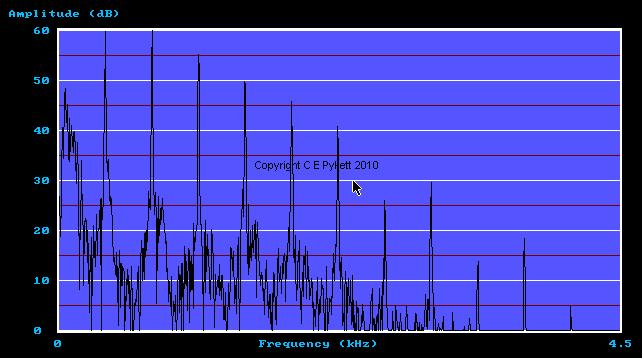
Therefore I have devoted much effort over many years to the problem. An example of the frequency spectrum of a very noisy raw sample is shown
in Figure 1. This relates to a
trumpet pipe in the middle of the keyboard in which not only the harmonics but
the intrusive blower noise (the grass between the harmonics) can be seen.
The sample can also be heard by clicking on the mp3 link below:
Figure 1. Example of a very noisy trumpet spectrum Blower noise is a mixture of the racket kicked up by the motor and fans,
accompanied by assorted rushing and hissing sounds.
The picture is a good illustration of the assertion made earlier that
blower noise generally increases markedly towards the lower frequencies and
falls away towards the higher ones. In
this case it decreased by about 46 dB over a 3.5 kHz frequency range, a factor
of 200 in amplitude. Unlike some
blowers, this one generated mainly random noise; it showed no evidence of
discrete frequencies at the fan blade rate or other periodic artefacts.
(As a counter-example, some years ago you could hear the blower at
Lincoln cathedral humming away noticeably in the building at 50 Hz, to the
extent it generated an objectionable 1 Hz beat whenever bottom G on a quiet 16
foot stop was played! It even
exists on a CD of the Lincoln instrument produced by a well known firm, though
they refused to admit it. Whether
the situation has improved since then I could not say). Outband noise reduction - high and low pass EQ One simple way to reduce noise, sometimes quite a lot of it, is to use a
high pass filter with a breakpoint or knee just below the fundamental frequency
of the sample. In other words one
applies bass cut or EQ because there is absolutely no reason to allow outband
noise below this frequency from any source to contaminate the sample.
The filtering can be done by computer in a waveform editor after the
samples have been recorded, but I sometimes prefer to use an analogue filter
inserted between the microphone and the recorder input while making the
recording. A second order (-12
dB/8ve) filter is more effective than a first order one (-6 dB/8ve), and a
variable cutoff frequency is of course necessary to match the filter knee to the
pipe being recorded. The advantage
of ‘pre-whitening’ the spectrum by analogue equalisation in this way is that
high amplitude blower noise at low outband frequencies does not then dominate
the recording level. This makes it
possible to use a higher gain setting than would otherwise be feasible.
As discussed above, this can be particularly beneficial when sampling
quiet pipes so that their full harmonic retinue can be captured with a high
enough signal to noise ratio. However the technique cannot be used for very low
frequency pipes of course, because there is not enough room left at the low end
of the frequency spectrum (below the fundamental) for the filter roll-off to be
effective. But apart from a few
cases such as this, high pass filtering should always be considered as a first
step in noise reduction.
Low pass filtering or treble cut EQ can also sometimes be used at the top end of the frequency band if the highest harmonic of the waveform sample is well below the frequency limit of the recording system. This will often be the case for quiet flutes, especially low pitched ones. However unlike bass cut, it is not safe to apply this form of EQ using an analogue filter prior to the recorder, because one has no knowledge at that time of the highest frequency in the sample. It can only be done after viewing a frequency spectrum of the recorded sample and making a judgement on that basis. Frequency domain noise reduction More sophisticated techniques are necessary to further reduce the noise
however. Any waveform editor worthy
of the name will incorporate a noise reduction option in its toolkit, and it is
necessary that you have available a few seconds of noise (only) recorded before
you keyed the pipe being sampled. The
noise reducer first derives the frequency structure of the noise and then
subtracts it from the spectrum of the sample on a frequency by frequency basis,
that is by operating in the frequency domain.
In theory this will then leave only the desired noise free sample.
In practice things do not always quite go to this plan however, and
audible noise might still remain on the ostensibly denoised sample waveform.
The reason why this happens is that this type of noise reduction assumes
that the noise is statistically stationary, which means that its average power
at each frequency remains the same at all times.
This is true for noise produced by a strictly random process such as
white or pink noise, but it is often not true for blower noise. This is frequently ‘lumpy’ in character in which audible
pulses of noise seem to occur unpredictably.
Furthermore, denoising a waveform on which a chuffy tremulant has been
imposed can be next to impossible using this method. However, unless the result is worse than before (and it can
be), standard denoising should always be tried. A tracking comb filter optimised for virtual
pipe organs Beyond this I use another method which completely – and I mean
completely – removes all trace of noise.
It relies on the fact that the subjective perception of noise arises
because of its continuous frequency spectrum, as opposed to that of the signal
which is peaky at the harmonic frequencies only. These distinct characteristics are used by our ears and brain
to distinguish between them and thus assign them different cultural names
(‘music’ and ‘noise’). For
example you can see from Figure 1 that there is appreciable (i.e. visible) noise
power at all frequencies from zero frequency up to about 3.5 kHz within the
dynamic range of the graph, and thereafter it continues falling off to yet
higher frequencies. Except below
the fundamental, where it does not matter very much because it can be
significantly reduced by high pass EQ, the noise is at least 40 dB down on the
highest amplitude harmonics (the first two in this example). Minus 40 dB is a ratio of one hundredth in amplitude and a
minute one ten-thousandth in power, so why does noise at this low level sound so
intrusive in this sample? The
reason is that the total noise power integrated over the entire audio
band is substantial, and it is this which the ear latches onto.
But because the desired signal only has power at its harmonic frequencies
as shown by the sharp spectrum lines, we can throw away anything existing
between them, and this includes the vast majority of the noise. Some years ago I developed a technique to do this.
It began merely as a tool to assist in capturing the amplitudes of all
the harmonics in a signal, which is otherwise tedious and error-prone because
one would have to read them all off manually one by one from a spectrum plot.
The operation of the tool is illustrated in Figure 2, which shows another
acoustic spectrum of an organ pipe but this time with its harmonics identified
by the small red circles. The
program which achieves this has to be led by the nose at first because you have
to click with the mouse vaguely near the fundamental frequency, whereupon the
computer identifies this peak precisely and then those of the harmonics. Having done so it then draws the circles to allow you to
judge whether it has been successful in seeking out the peaks in the plot
(occasionally it is not successful and then you have to try again).
When you are satisfied it then sends these numbers (the amplitudes and
frequencies of all the harmonics) to a file for storage
and further processing. Figure 2. Illustrating automated harmonic capture Initially I used this program only for additive synthesis purposes,
because the harmonic values can be used to resynthesise a waveform using the
fast inverse Fourier transform (IFT). However
the important point is that the waveform thus synthesised is completely noise
free when auditioned, because everything in the spectrum was discarded except
for the peaks of the harmonics, and we have already seen that the vast majority
of the noise power exists between the harmonics. Unfortunately, although the resynthesised waveform is indeed
subjectively noise free, it has other major shortcomings.
The principal one is that all of the ‘live’ character of the original
sound is lost because the spectrum from which the harmonics were captured was
derived only from a single snapshot of the
signal, a short piece of its waveform during the sustain phase.
The liveness in the
original waveform arises from small variations in the amplitudes and frequencies
of the harmonics of the pipe as it reacts to diverse phenomena such as unsteady
winding while the note was being sustained as the key was held down. Another problem is that
the attack and release transients, including the reverberation tail in the
recording room after the pipe ceases to speak, are also lost.
Fortunately these missing features can be recovered, at least to some
extent if not completely, by capitalising on the fact that the peak-finding
algorithm described above is (slightly) intelligent – as just outlined,
it can find a nearby spectrum peak on its own if it thinks it has not
quite got there. What one does in an extended version of the program is first to encourage it to find the spectrum peaks as before at an arbitrary point well inside the sustain (steady state) region of the waveform sample. Having done this the program then tracks forwards in time along the recorded waveform sample on its own, following the harmonics as they move around slightly in amplitude and frequency. This forward-track process continues automatically until it terminates at the end of the sample when room ambience has died away. A similar back-track process is also undertaken in which the program moves backwards in time from the original start point, through the attack transient to reach the start of the sample. The set of numbers thus derived in effect describe the complete attack-sustain-release history for each harmonic or partial in terms of its (small) amplitude and frequency variations. These can therefore be used in a more sophisticated but nevertheless standard additive synthesis algorithm to resynthesise the complete waveform sample. Several tools exist which can do this. (If one is using an additive synthesis sound engine, the time histories could simply be fed into it because no off-line resynthesis of the denoised waveform would then be necessary. However no VPO currently uses additive synthesis to the best of my knowledge). This version of the sample will now contain no noise but it will retain an approximation to the original attack and release transients plus the liveness of the sustain phase. The process works better with some samples than others, but there are several parameters which the user can tweak to try and improve performance in difficult cases. Some heuristic tricks are employed to optimise the performance of the technique, and again these are specific to the VPO scenario. For example, the amplitude and frequency of each partial or harmonic of an actual organ pipe will not move too far while it sounds (unless it is tremulated), thus the program can self-correct or flag anomalous estimates as it moves along the waveform. What has just been described is an example of the application-specific processing techniques for VPOs which I alluded to at the outset. It takes advantage of the markedly different characteristics of noise and signal in the frequency domain for a VPO in that their respective power distributions differ considerably. In signal processing parlance it could be described as an extremely high-Q tracking comb filter, that is one with extremely sharp 'teeth' whose width does not exceed that of one frequency bin of the spectrum. Moreover it has no stopband ripple in the inter-harmonic regions between the teeth, and the stopbands are as deep as the dynamic range of the spectrum itself. It also has a further capability beyond this in that the frequencies constituting the teeth do not necessarily have to be exact harmonics of the fundamental. While exact frequency relationships will be maintained during the sustain portion of the waveform sample while the forced harmonics of the pipe are in control, the frequencies might diverge slightly during the attack and decay transients when the natural partials dominate its speech. The algorithm is designed to detect this behaviour. Also, because it removes all trace of noise, the process is particularly useful with 'wet' samples which capture the ambience of the recording room as an extended reverberation tail. With other forms of noise reduction, releasing a full chord on a VPO will sometimes reveal the presence of residual noise on wet samples as a sort of transitory hiss as they decay into inaudibility, even though little or no noise can be detected on the individual waveforms. This is because the smallest amount of noise on each sample builds up additively when the VPO is played to the extent it can sometimes become momentarily audible when the keys are released. Summarising, noise on a waveform sample can be reduced in at least three
ways, which I usually use and in this order: outband noise reduction using high and low pass EQ, standard
wideband noise reduction methods and finally VPO-specific techniques such as the
tracking filter described above. Two issues which crop up repeatedly when preparing waveform sample sets
for virtual pipe organs are the bit depth which should be used when making
recordings of organ pipes, and how to subsequently remove noise from them.
It was shown that the dynamic range of individual organ pipes extends
from the pipe with the greatest SPL (not necessarily the same as the
subjectively loudest one) to the weakest harmonic of the pipe with the smallest
SPL. An example was given of an
organ whose dynamic range lay within that of a 16 bit recorder but without much
of a safety margin. Therefore it
was suggested that at least 20 bits or so would be a more realistic working
minimum, though this could be reduced by judiciously varying the gain to match
the level of the sample being recorded. Noise on the recorded samples is dominated by the organ blower, and it
was shown how the noise could be reduced in three ways:
high and low pass filtering below the fundamental frequency and above the
highest harmonic (respectively) to reduce outband
noise, conventional frequency domain subtractive noise reduction, and the
application of VPO-specific tools. A
specially developed tracking comb filter was described which is effective in the
latter case; this capitalises on the different power distributions of noise and
signal as a function of frequency - noise exists at all frequencies across a
significant part of the audio spectrum whereas the wanted signals have their
power confined to well defined harmonics. This
difference enables the amplitude and frequency of each harmonic or partial to be
tracked automatically from the start of the attack transient of the sound, and
then through the sustain phase to the end of the release transient.
Because power at all other frequencies is ignored, the result is
completely noise free. 1.
The virtual pipe organ uses the massive
processing power and memory of modern personal computers, and multimedia devices
such as sound cards, to render the desired sounds in response to MIDI commands
from the player at some form of console. VPOs
currently use sampled sound synthesis as opposed to additive synthesis or
physical modelling techniques. These
methods are described in [2] below, together with several other background
references available on this website. A
VPO will typically accommodate a separate sound sample for every note of every
stop, each sample being up to several seconds in duration in some cases.
By no means all commercial digital organs are able to do this. Most VPO software is free, and some of it is also supported by active user groups. Some of the associated source code is open-sourced as well. Note that availability of the software does not imply that an item is still actively supported though. This article is not an advertisement for any particular VPO and it does not imply a recommendation for it, as mentioning products by name would be invidious. However having said that, most if not all of the items have in some way contributed to the ascendancy of the VPO over the last decade or so and they have therefore helped to shape it into the popular and valuable musical resource it is today. 2. “Digital Organs Today”, Colin Pykett, Organists’ Review, November 2009. Also available on this website (read). Other articles on this site amplify some technical aspects of VPOs in more detail: “Voicing electronic organs” (read) “How synthesisers work” (read) “Wet or dry sampling for digital organs?” (read) “Physical modelling in digital organs” (read) “Tremulant simulation in digital organs” (read) “Digital organs using off-the-shelf technology” (read) 3. “The mysteries of organ sounds – a journey”, C E Pykett, 2011. Available on this website (read).
4. "The Tonal Structure of Organ Flutes", C E Pykett, 2003. Available on this website (read).
|