


|
|
|
The Mysteries of Organ Sounds - a journey
by Colin Pykett Posted: 23 March 2011 Last revised: 1 January 2021 Copyright © C E Pykett
"He that travelleth into a country before he hath some entrance into the language, goeth to school, and not to travel" Francis Bacon
Abstract. This article uses the narrative device of a personal journey occupying half a century to illustrate how advances in digital technology have influenced the way organ pipe sounds are analysed and embedded in electronic organs. It begins with the huge and expensive batch-processing bureau computers of the 1960's which were largely inaccessible and irrelevant to the majority of those in the electronic music field, and ends with today's personal computers which can host cheap virtual pipe organs whose sound quality can exceed that of commercial products costing many times as much. The article concludes by pondering on how this might affect a trade already suffering from the impact of a contracting market.
Contents (click on the headings below to access the desired section)
Spectrum analysis at home - still the 1970’s
Into the Windows era - the 1990’s
The new millennium - websites and virtual pipe organs
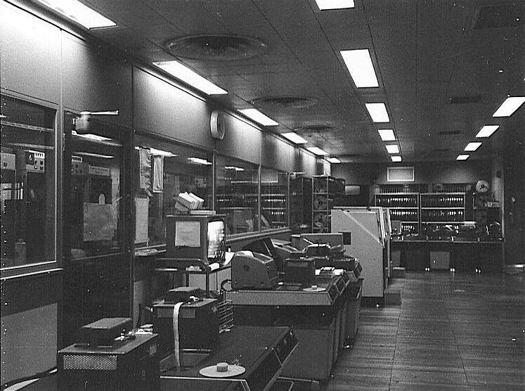
Younger readers arguably should not bother with this article. If you are less than about thirty you may never have heard an early Allen digital organ, let alone some of the impressive analogue instruments by firms such as Copeman Hart [1]. Also you may not remember a time when people did not have computers at home either. Only those whose recall extends further back to the days when both computers and electronic organs were huge, rare and expensive might conceivably find something to interest them here. The reason for mentioning organs and computers in the same breath is twofold. Firstly, it had been tedious to the point of impossibility to analyse the sounds of organ pipes in the necessary quantity and detail until computers became available to the average user. Such analyses were necessary to understand their physics, which then fed into the design of improved tone production in electronic organs. Secondly, as costs and sizes came down, the computer technology itself gave birth to the field of digital audio in general and digital organs in particular. These twin benefits of improved acoustical understanding and more accessible digital technology also resulted in changes to pipe organ building in terms of voicing and control systems. It was coincidental that I began having organ lessons and first met a computer in the 1960’s, so I can tell this story in terms of a personal journey across a landscape of continually improving capability and decreasing cost, both for computers and organs. Hence the title of this article. Therefore please note that it is purely my personal story, not a historical survey of the development of digital organs. My work is also continuing in fields such as software synthesis and physical modelling, so the account remains interim rather than complete. I still recall the day in 1965 when I first attended a computer programming course while reading physics at London university. They had recently installed a Ferranti Atlas computer, only the second one made. It was then one of the fastest in the world, if not the fastest, with an addition taking typically 1.5 microseconds. At least it was built with transistors though, not valves. There was barely 1 MB of memory, yet it cost a six figure sum in pounds sterling, consumed power measured in kilowatts and filled a huge air conditioned room (Figure 1). Thus the machine was around 3000 times slower than a typical laptop today and its memory was 20,000 times smaller. Those were the days of computer bureaux, built around huge batch-processing machines rather than today's PC's. You were not allowed to use such computers yourself, indeed you could not enter the room. Your programs, punched on paper tape in the case of Atlas, were whisked away by ‘operators’ with a superior attitude akin to that of doctors’ receptionists. If you were lucky you might get the results back the same afternoon, but usually it was the following day. More often than not the program had not even compiled, let alone run, so you had to go through the whole process again - and again. Do not laugh too loud though; an even more primitive machine at London had decoded the double helical structure of DNA a decade earlier [2].
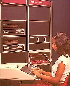
Figure 1. The Atlas computer room at London university c. 1965 (© STFC Rutherford Appleton Laboratory. Picture by Bill Williams) Although I was playing various organs in London at that time and was interested in the physics of organ pipes, I was not able to use Atlas to analyse their sounds. Not only would it have been forbidden, it did not occur to me. Even if it had, the problems were many. For instance, how could I have got the sounds into the computer in the first place? For such reasons, doing things like deriving the harmonic structure of musical sounds were routinely achieved using analogue methods in those days. However the necessary analysis equipment was so expensive it sometimes could not even be afforded by university research groups, let alone impecunious individuals such as myself. So things stalled for a decade until the mid-1970’s, when I persuaded my then-employer to invest in a so-called minicomputer. This was a PDP-11 made by the Digital Equipment Corporation (DEC) and, unlike Atlas, it belonged solely to me and my research group. We used it for analysing radar signals and the like and it occupied several six-foot-high cabinets, again in an air conditioned room but a much smaller one than that in which Atlas had reposed (Figure 2). To be fair, the contents of the cabinets was mostly fresh air and I wonder to this day why they were so large. Maybe it was a marketing issue in that the ad-men still thought computers had to look large and fearsome so that customers would think they were getting their money’s worth. The machine had 64KB of memory and was about the same speed as Atlas, but at £40,000 it was much cheaper. In purely arithmetic terms its speed was much enhanced because I had specified the inclusion of a hardware floating point arithmetic co-processor. Figure 2. A DEC PDP-11/40 minicomputer The
processor itself was the small module with the row of key switches in the right
hand cabinet, and two removeable
disks can be seen in the left hand one (1.2 MB capacity each).
Our machine also had another rack housing a digital tape deck. Besides its speed, another notable feature of the PDP-11 was its analogue-to-digital converter (ADC) which enabled signals from the outside world to be digitised and stored within the computer, and this led me to think of using it to analyse the sounds of organ pipes. Indeed, Peter Comerford’s team at Bradford university was using a similar PDP-11 to do exactly that as part of their development of the Bradford Computing Organ, and I visited him around this time to try an early prototype. So after some cajoling my employer granted me a concession to use our machine, one time only, to analyse my library of organ pipe recordings which existed on analogue tape. This gave a tremendous boost to my understanding of the physics involved. An example of the results obtained is shown in Figure 3, which shows the harmonic spectrum of a pipe from a 4 foot principal stop. The sounds of hundreds of other pipes were analysed in the same way during that session.
Figure 3. Frequency spectrum showing the harmonic structure of a small principal pipe obtained using a PDP-11 minicomputer Spectrum analysis at home - still the 1970’s After that my appetite was whetted for more of the same, but because further access to the computer at work was not possible I started to develop some analysis gear of my own. In the 1970’s the idea of other than a toy computer at home was meaningless because one having the necessary capability did not exist at any price. Even so basic a machine as the Sinclair ZX81 was still some years away, and it would have been totally inadequate in any case. So it was back to the drawing board, and I developed two pieces of kit which saw untold hours of use. One was an electronic memory which would store a short sound sample of the pipe being analysed, and the other was a scanning filter which then revealed its harmonic structure. Both were functionally similar to some expensive laboratory items which were marketed by firms such as Marconi Instruments and Bruel & Kjaer at the time, though (incredibly) these still used valves. At least my home-brewed designs had moved into the solid state era.
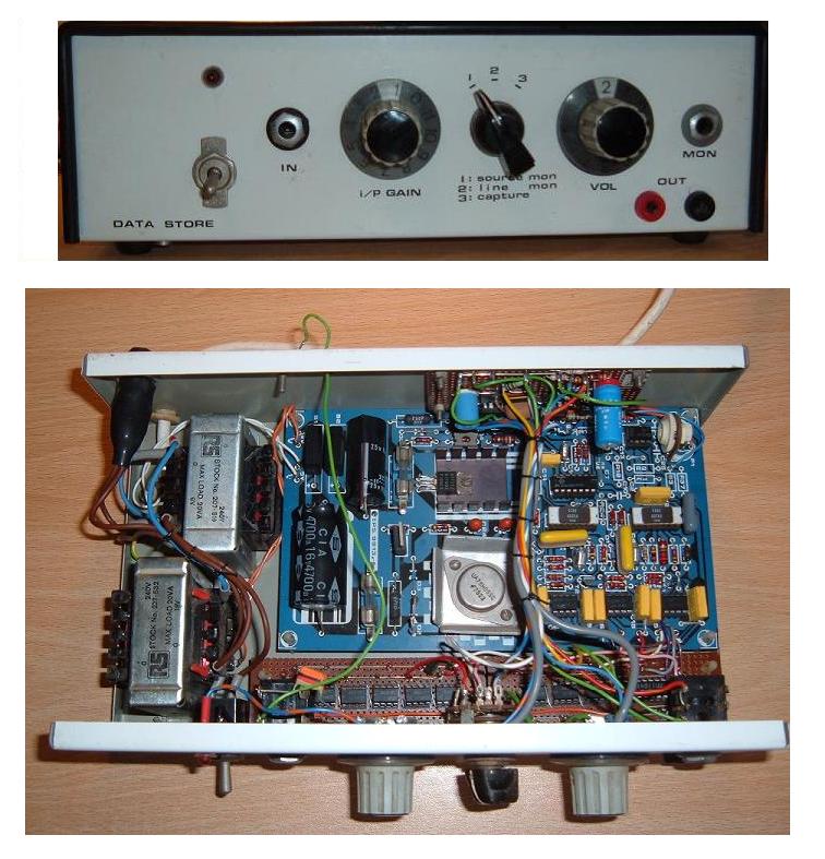
Figure 4. Recirculating data store
The memory unit was a recirculating data store and it is shown at Figure 4. First of all it digitised a sample of the organ pipe sound, either directly from a microphone in the building or from a recording on analogue tape, and then it stored the sample in a long shift register memory. Secondly it would read out the stored sample continuously and output it as an analogue signal through a digital to analogue converter (DAC). In functional terms it was therefore rather like a continuous loop of recording tape, but it had the advantage of never wearing out. The analogue output from the data store was applied to the second piece of kit, a harmonic or wave analyser (Figure 5). This used a high-Q filter which was, in effect, manually scanned across the frequency range of interest. However the filter itself was configured as a heterodyne filter. This means it was tuned to a fixed intermediate frequency, the scanning being done by multiplying the incoming signal with a variable frequency sine wave from a BFO (beat frequency oscillator). All the harmonics from the organ pipe in the input signal were thereby shifted into sideband frequencies via a process of suppressed carrier amplitude modulation. When one of these sidebands coincided with the fixed frequency to which the filter was tuned, an output was obtained.
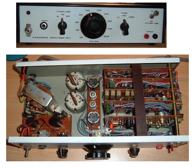
Figure 5. Harmonic Analyser
The amplitude of the filter output was proportional to that of the harmonic currently being analysed in the original input waveform. When rectified, this signal was applied to a DC voltmeter (not shown in the picture) - you plugged the meter into the red and black sockets on the front panel. So by turning the large knob in the picture you could scan for harmonics across any desired frequency range, and it was somehow very satisfying to see the meter needle rise and fall as you tuned through them. It was admittedly a somewhat tedious way to derive the spectrum of an organ pipe, but it produced very accurate results. The dynamic range (signal to noise ratio) was high at over 80 dB, equivalent to a 13 bit digital processing system, because of the very narrow bandwidth (a few Hz) of the high-Q heterodyne filter. This figure was much higher than that of the original sound picked up by a microphone because of the extraneous noises always encountered when making organ recordings, particularly those caused by the organ blower. It was also much higher than than any analogue tape recorder, which would struggle to reach 60 dB on a good day. In practice it meant that you could pull a surprisingly weak harmonic out of a very noisy signal. The managing director of more than one well known electronic organ firm beat a path to my door in those days to see the system. At that time there were few alternatives available to those who could not afford a minicomputer (i.e. just about all of them), and one of these firms was capturing organ pipe waveforms on the tube of a storage oscilloscope rather than in a digital memory as I did. I cannot recall how they then proceeded to analyse the frequency structure though. And so another decade passed, bringing us up to the mid-1980’s. During this period I had published a study in the technical literature describing a design methodology for tone formation in electronic organs based on real pipe sounds [3]. This used results from the research outlined above. I had also incorporated this method of tone production into a prototype electronic organ which can be seen in Figure 6.
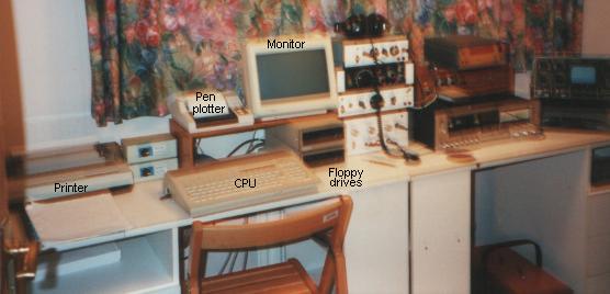
Figure 6. First electronic organ using tone production based on real pipe sounds (1984) This instrument was quite satisfying and it, too, was visited by various organ builders. One of these wanted to incorporate my designs into an instrument which he was to exhibit at the St Albans organ festival that year, but unfortunately he didn’t want to pay anything for them! Tight or what? You can guess what my answer was (it was fairly dusty). Although there were a few very good commercial analogue organs around at that time, notably those by Copeman Hart here in the UK, they were expensive and difficult to make. Thus they were already a dying breed, particularly as several firms were now beginning to expand into the new field of digital instruments. Examples included Copeman Hart themselves, Wyvern and Ahlborn, all of whom used the digital additive synthesis technology based on that invented at Bradford university around 1980 and subsequently modified by Musicom. Because of this evolving situation I had an article accepted for publication in the prestigious journal Musical Times, dealing with what to look for in both analogue organs as well as the burgeoning digital field [4]. I also started to consider whether I could enter this field myself without having to spend too much money, and this meant looking at the then-embryonic field of home computing. At this point things really started to hot up. The IBM PC had already made its debut in 1981, but it was rather an unattractive beast for audio purposes as well as being expensive for what it was. However its appearance resulted in the simultaneous availability of several competing products at rock-bottom prices on the surplus market. This fortuitous event happened because IBM had decided to brutally kill off the competition by putting the design of its new PC into the public domain, thereby inventing the PC clone concept because it could be widely copied, and the only firm which survived this onslaught was Apple with their Macintosh. However the early Mac’s, too, were unattractive for audio work because their limited processing power was largely swallowed up by their admittedly attractive user interface, which Microsoft later competed with in Windows. So I bought one of the cheap surplus casualties of this iconoclasm, a Triumph-Adler office computer called the Alphatronic. Like many other brands at the time, it used a Z80 processor and the CP/M operating system. It was good value because it also came with two floppy disc drives, making it very useful and flexible as regards storing organ pipe waveforms. The Alphatronic ran at 4 MHz and it had 64 KB of memory. On paper it was therefore about as powerful as the PDP-11 of ten years earlier, although it did not have the luxury of a floating point co-processor so it was slower in arithmetic terms. But it only cost a tiny fraction of the price and it was only a tiny fraction of the size. It can be seen in Figure 7 in the analysis studio I set up at home (not a very good photo unfortunately).
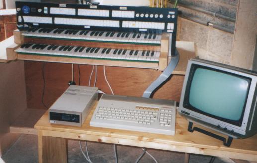
Figure 7. Home waveform analysis lab in the 1980’s showing the Alphatronic (Z80) computer setup plus the other gear referred to in this article The Z80 processor chip had been chosen a few years earlier as the nucleus of the Bradford organ system, and the Alphatronic made a very satisfactory Z80 software development system for my own digital organ work. Z80 computers using the CP/M operating system were well supported at that time, particularly by Microsoft before the vast potential of the IBM PC software market opened up to them. I programmed in Fortran, Basic and Z80 assembler language depending on the needs of the job, using Microsoft products in each case. That their Fortran compiler existed at all was a miracle, considering the tiny memory and disc capacities. Yet this was before the days of software bloat. Although the Alphatronic was a command line machine with no fancy GUI (it had a user interface similar to MS-DOS) it booted in about 5 seconds flat, and it would compile and link a typical Fortran program in under a minute. When watching egg-timers, rotating circles or beach balls for minutes on end on today’s computers (not to mention freezes and BSOD’s), I sometimes cannot help thinking something has been lost along the way. The Alphatronic turned out to be so useful that I bought several others even more cheaply and used them in an early experimental digital organ (Figure 8). Today, I regret having thrown all of them into a skip as they are apparently sought after on the vintage computing market, and it would be nice to think they had found a better home.
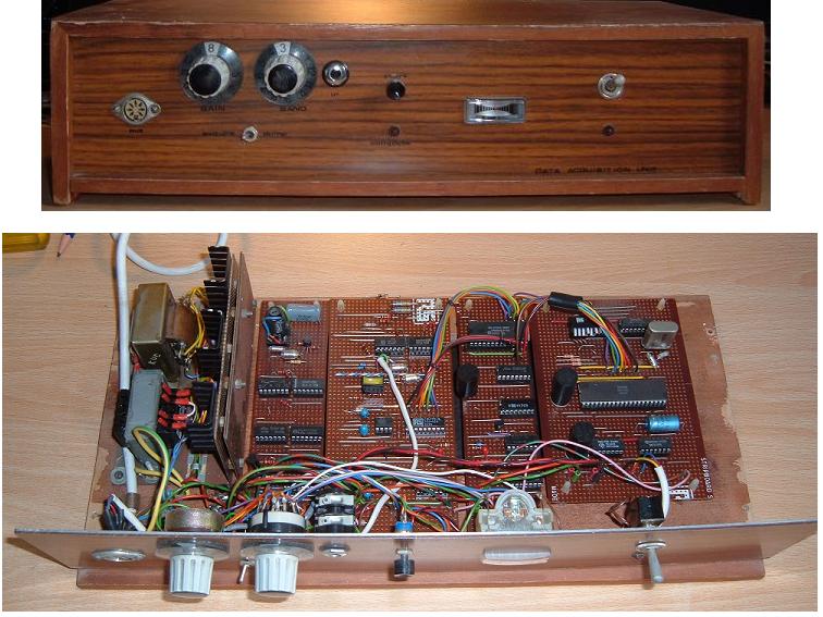
Figure 8. An Alphatronic (Z80) computer driving an experimental digital organ However, the main downside was the one thing that the Alphatronic machine did not have - an ADC. So until I did something about this I could not get sounds from the outside world into the computer with the intention of analysing them. ‘Sound card’ was a term which did not exist at that time, even for the IBM PC, so again I had to design and build yet another add-on box of electronics - a data acquisition unit this time (Figure 9). It was one of the first things I did after acquiring the Alphatronic.
Figure 9. Data acquisition unit for the Alphatronic (Z80) computer The reason for using the unnecessarily fancy (though battered) wooden box was that it was just sitting around, having formerly housed an old FM radio tuner. The unit comprised an ADC which stored a digitised sample of the input waveform in an SRAM memory. The waveform was of course from an organ pipe, usually recorded on analogue tape. The stored sample was then read out digitally from the DIN socket on the front panel into the serial port of the Alphatronic computer, and retained as a floppy disc file. Any number of signal processing operations could then be performed on this file, such as spectrum analysis. A nice example is shown in Figure 10, which is a 3-dimensional time/frequency/amplitude plot (sometimes called a spectrogram) of how a flue pipe comes onto speech. The programs which produced this plot, including the FFT subroutine and the hidden line algorithm to generate the 3-d effect, all had to be written from scratch. Such software was rare and expensive in those days even if you could obtain it, so it was much cheaper and often quicker to write one's own.
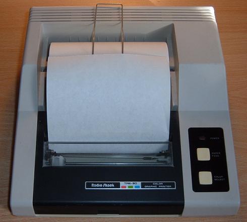
Figure 10. A time-frequency spectrogram of a flue pipe coming onto speech This picture was actually plotted using a neat little Radio Shack pen plotter, again driven using bespoke software. Although long obsolete, this remains such an attractive device that I still use it from time to time, having written drivers to run under Windows on modern PC’s. Thus you will observe that it did not follow the Alphatronic machines into the skip! It plots in up to four colours using tiny ball point pens. It can be driven either from a serial or a parallel port and it can be seen in the earlier picture of my waveform analysis setup (Figure 7). A closer view is at Figure 11.
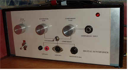
Figure 11. Radio Shack four-colour pen plotter type TRS-80 Because the Alphatronic computer was also used to generate sounds for digital organs as well as analysing them, I designed a further add-on unit to assist in voicing. This was a hardware synthesiser which accepted any waveform from the computer and then read it out repetitively in the form of a periodic audio sound at any desired frequency. Again, this was necessary because sound cards were still things of the future. It was controlled from the parallel port of the computer and is shown in Figure 12.
Figure 12. External hardware synthesiser - the port for connecting to the computer is at the rear This unit has some bespoke features which are so useful to a digital organ voicer that I still use it today (2018) with modern PC’s. One such feature is a simple hardware one - the ability to connect the original recording of the organ pipe being analysed to the ‘comparison input’ of the synthesiser and adjust its volume. By switching from this signal to the synthesised version it is then possible to assess how successful the synthesis has been. By repeatedly switching back and forth between the two waveforms while adjusting the synthetic one, extremely accurate reconstruction of organ sounds can be achieved - the toggle switch which can be seen in the centre of the synthesiser's control panel is used for this purpose. Incidentally, one lesson learnt was that our ears (at least, mine) seem unable to accurately match the timbres of two sounds (that of a real organ pipe and its simulated version) unless their pitches and volumes are identical. Even small differences will otherwise distract the ear and prevent an exact correspondence of tone colour being achieved. This is the reason for the three knobs on the synthesiser, two of which are gain controls while the third fine-tunes the pitch of the synthesised waveform to precisely match that of the original recording. Another feature is the way the unit integrates with the software I wrote to control it. For instance, one program throws up the spectrum of an organ pipe on the screen as a graph of the sort shown in Figure 13. It is only necessary to click when the mouse pointer is placed somewhere near the fundamental to enable its amplitude and that of all the other harmonics to be found automatically. They are identified by the small red circles, and their values can be used to synthesise a waveform using additive synthesis. This waveform can then be zapped into the memory of the external synthesiser so you can hear it.
Figure 13. Spectrum analysis program showing how harmonics are automatically detected (the small red circles) Another program enables real time adjustments to be made to synthetic waveforms, for example by changing the amplitudes of selected harmonics. The screenshot below (Figure 14) shows how a spectrum can be modified interactively and the results auditioned in real time via the synthesiser. The spectrum (i.e. the harmonic amplitudes) will typically have been obtained automatically from the spectrum analysis program described above, or they can be inserted manually from scratch if you want to try "inventing" a new sound. In this display the 3rd harmonic of a 16 foot Violone pipe has been adjusted from its original value to one of 45 dB, and it is shown in the display as a red line for this reason. Each time such a change is made, an inverse Fourier transform is performed automatically (additive synthesis) and the result loaded into the synthesiser. The speed of the system is such that the new sound is heard immediately. A MIDI keyboard can be connected if desired so that the effect of "spreading" the spectrum across a keygroup can be assessed. However a simpler option is also available in which the numeric keys on the computer keyboard can be used for the same purpose to allow the frequency of the note to be shifted semitonally over an octave. To activate this option this one simply clicks the 'keyboard' button seen on the display. The octave in question is selected by means of the 'octave' and 'footage' buttons on the screen.
Using this program it is possible to optimise the various spectra used for an organ stop across the keyboard compass, and to define the voicing points (keygroups) as well if they are used. The program is equally applicable to time domain and frequency domain synthesis - for the former, the spectrum of the sampled waveform is first obtained rapidly using the spectrum analysis facilities described above. Once the results of modifying the spectrum are satisfactory it can then be re-transformed back into a time waveform for use by a time domain organ system. In passing, it should also be noted that it is virtually impossible to develop the necessary voicing skills without a tool of this type. Only by learning how the timbre of a sound depends on its harmonic structure, and how this dependency varies dramatically with pitch and with the type of spectrum (flute, reed, etc), is it possible to voice an electronic organ effectively.
Figure 14. Interactive voicing program showing by the red line how individual harmonics in a spectrum can be selected and adjusted
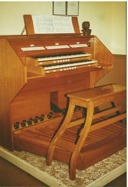
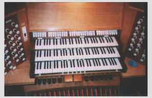
This system of synthesis hardware integrated with bespoke software provides a slick way of assessing how well one’s synthesised waveforms compare to the original pipe sounds. However, before some of the later programs could be written, it was necessary to wait for the best part of yet another decade until Windows had matured and until computers became fast enough. So this part of the story follows next. In the meantime though, I expanded the organ shown earlier to three manuals with a wider choice of stops (Figure 15) to capitalise on the latest improvements which had resulted from my recent research. This was completed in 1988, and you can hear something of the results I was achieving twenty-plus years ago by clicking here.
Figure 15. Later three manual organ incorporating updated sound generation techniques (1988) Into the Windows era - the 1990’s As we entered 1990 the IBM PC had been around for nearly a decade, and I now had to take it seriously as a candidate for the next step along the road. Windows 3.1 was available, but things were still by no means cheap and this was why I hung onto the Alphatronic setup for some years. However in 1992 V-Tech were the first to bring out a complete Windows PC system with an Intel 486 processor, the predecessor of the Pentium 1, for exactly one penny under £1000. Although this was an awful lot of money in those days, it came with a lot of attractive software and a monitor and so it worked straight out of the box. Having taken the plunge, I now had a machine at home which was more advanced than most of those at work for the first time in my life (they were mostly still making do with 386’s), and I was very pleased with it. The family liked it too, so much so that there were the usual domestic squabbles as to who was going to use it first after tea that evening. (However this did have the advantage that one could use it as a lever to get rooms tidied, homework done, etc). It was about six times faster than the old Z80 system, it had vastly more memory and of course the pleasing Windows 3.1 user interface. But it still had major shortcomings for digital organ work and audio in general, because sound cards with anything beyond a laughable capability had yet to make their appearance. Consequently functions such as digitising audio waveforms and sound synthesis still needed specialised add-on hardware such as that I had built for the Alphatronic computer. Therefore I retained these units even though we were now in the Windows era. Getting them to work with the new PC required the associated software to be re-coded however, which was a major undertaking. Fortunately the hardware interfaces had not changed because the IBM PC had ports which were pin-for-pin compatible with those of the Alphatronic. When Windows 95 hit the streets a few years later I hung back. The horror stories turned out not to be mere teething troubles but a raft of continuing problems, so I decided to stick with Windows 3.1. A few more years later the first appearance of Windows 98 was little better until Windows 98SE superseded it. But, although still far from perfect, it was time to consider trading up for another reason - the appearance for the first time of decent sound cards. The SoundBlaster Live from Creative Labs, followed by the Audigy, did at an economic price what my former collection of add-on boxes had done faithfully for some fifteen years, particularly as regards digitising waveforms and sound synthesis. However I still continued to use the old hardware for certain purposes, and occasionally do so today. The 1990’s had been an interesting decade. My early work on digital tone production with the Alphatronic computer had continued and become more sophisticated with the transition to the more powerful Windows PC’s. On the commercial front there had been an explosion in the number of firms offering digital organs using stored sound samples once the Rockwell patents (used by Allen) expired. So as the millennium drew to a close I published another article, in Organists’ Review this time, which updated the one in Musical Times eleven years earlier to cover the expanding digital organ field in more detail [5]. The new millennium - websites and virtual pipe organs Armed with my latest Windows 98 PC in 1999, I put the first version of the website you are now visiting on the web. (Yes, I realise the new millennium had not quite started then but it was close enough). It was slow going though, literally, considering that a broadband Internet connection was still a few years away where I lived. Thus the whole thing had to be done via dial-up at first. Nevertheless the site has remained live ever since. Once the new millennium got under way I realised how prophetic were some words I had used in the Organists’ Review article a few years earlier [5]. They read:
The italics have been overlaid deliberately here - read on to see why. Everything in this statement was true at that time, but having obtained the first Audigy sound card when it appeared only a year or so later, I recall looking at it and thinking that it was nothing less than a small but complete sound engine for a digital organ. Using today’s vernacular, it could be considered as a 64-note music module for such an instrument. Therefore I reasoned that by using enough such cards, one could construct a complete PC-based instrument of any reasonable size fairly cheaply. The difference between commercial organs and this new approach was not one of principle but of implementation, because most of them used stored sound samples in much the same way as the wavetable synthesisers in the Audigy. However the use of off-the-shelf hardware in the form of sound cards and PC’s would remove the need to develop the type of expensive custom sound engine that had been used hitherto by the trade. There were also other advantages. One was that, because the system used a PC, its vast memory could hold far more sound samples than any sound engine then in commercial use as far as I was aware. But this aspect also mandated the use of a recent sound card such as the Audigy, because this was one of the first to use the computer’s memory for waveform storage rather than the limited amount on the card itself. In practice this meant that one could envisage, for the first time, the use of one stored sound sample per note per stop, equivalent to the number of pipes in a pipe organ with the same stop list. Previously it was necessary to ‘stretch’ each waveform over a number of notes because of memory limitations, and most if not all commercial organs at that time did this. Many still do. Moreover, as memory sizes continued to grow as they were confidently predicted to do, the lengths of each sample could increase in proportion as the technology allowed. Using samples several seconds in length would remove the need to loop around only a few cycles of the waveform for notes of extended duration. These features would enable independent, long-duration samples to be used for each note, offering the prospect of much-improved fidelity in the sound of digital organs. However it was necessary to do quite a lot of programming to test these ideas because the sound cards were being used in a non-standard manner. They were largely aimed at gamers or home cinema enthusiasts, whereas I wanted to use them to build organs. The trick was to make the card think it was being driven by a MIDI sequencer such as Cubase, and it was also necessary to find a way to use several cards simultaneously. I used C and C++ for programming in view of its efficiency, having invested in Microsoft’s superb (but expensive) Visual Studio for software development. Nevertheless, the basic design was realised fairly quickly, and it was not long before a system with several sound cards was running. I called it Prog Organ (standing for Programmable Organ) because any number of different organs could be simulated and called up as required, and the design ideas which led up to it are described in more detail elsewhere on this website [6]. You can hear several hours of recordings made with the system here. By this time it was becoming apparent that others had been working along similar lines, and some products had even appeared commercially. One of the most famous was Marshall and Ogletree’s PC-based organ at Trinity Church, Wall Street in New York City in 2003. The name ‘virtual pipe organ’ (VPO) appeared around this time to distinguish products using this approach from the general run of instruments available in the trade. It was meant to indicate the availability of a separate, long-duration sound sample representing every pipe in an equivalent pipe organ. And so we have arrived almost at the present day after a journey which has lasted some 35 years, starting with analogue organs and analogue analysis gear long before home computers were thought of, and ending with VPO's running on today’s PC’s. Out of the blue, in 2009 I had a further commission from Organists’ Review who wanted an update to my previous 1998 article. So of course I had to include some discussion of VPO’s this time [7]. Largely because of the VPO concept, one striking aspect of the home organ scene today is its sophistication compared to that which existed 35 or so years ago. In those days the only way to get an electronic organ at home for most people was to go down the DIY route on account of the expense of commercial items, most of which were not very good anyway. Unfortunately, neither were the majority of the home made efforts, and their proud creators were not, on the whole, terribly clued up (bless them!). By contrast, even some quite modest and very cheap VPO’s today leave commercial products on the starting blocks in terms of the excellence of their sounds. And many of the VPO brigade are also extremely knowledgeable at the highest technical level, far more so than the average salesperson in a dealer’s showroom. This is obvious from their laudable practice of sharing their expertise freely on the Internet, which is also in stark contrast to the paranoid coyness of the digital organ industry at large. Therefore to call them amateurs is only permissible if one uses the word literally to mean one who loves the subject, rather than in its more usual pejorative sense. What all this means for the future of the traditional digital organ business implies watching an evolving and fascinating scene, because at least some manufacturers are obviously getting left behind both in terms of the technology they use and the results they achieve. (Some are still clinging onto Z80 or similar chips, and of these a very well known one has just gone to the wall as I write). As well as the competition from VPO’s there is a shrinking market for organs of any type, both piped and digital, and the obvious desperation of certain manufacturers was reflected in their belligerent reaction to my recent Organists’ Review article [7]. But let’s not go there. The more important conclusion here is that we should watch this space with interest! Thanks are due to STFC Rutherford Appleton Laboratory for the details and picture of the Atlas computer at London university. 1. Some historical milestones in the commercial digital organ field relevant to this article:
2. The power of today’s computers is largely swallowed up by their GUI - the pretty graphical user interface we see on a Windows or Mac PC with its coloured pictures and interactive capability. Together with the turgid slowness of any computer connected to the Internet, coupled with today’s bloated, inefficient, bug-ridden and nag-culture software, a modern PC does not have anything like the power one might expect from its bare performance figures. The end users, waiting patiently or otherwise for their results, are at the mercy of countless unwanted applications and the operating system itself whose designers, with their control-freak mentality, exercise complete dominance over any computer today for their own purposes. It takes time and know-how to remove such unwanted baggage from a retail PC before its power can be properly harnessed for purposes such as running virtual pipe organ programs. This explains why it was possible to solve the most complex problems on the much smaller but far more efficient machines of half a century ago. 3. “Tone Filters for Electronic Organs”, C E Pykett, Wireless World, October and December 1980. Available as a PDF file - 440 KB (download). 4. “Choosing an electronic organ”, C E Pykett, Musical Times, January 1987. Also available on this website (read). 5. “Electronic Organs”, C E Pykett, Organists’ Review, August 1998. Also available on this website (read). 6. “Digital Organs using Off-The-Shelf Technology”, C E Pykett, 2005. Available on this website (read). 7. “Digital Organs Today”, C E Pykett, Organists’ Review, November 2009. Also available on this website (read).
|