


|
|
|
Helpers and Haskells
Colin Pykett
Posted: 20 September 2022 Revised: 21 October 2022 Copyright C E Pykett
Abstract.
A stopped or closed organ pipe speaks an octave below the pitch of an open one
of the same length, but since the even-numbered harmonics are suppressed or
absent its timbre or tone quality is unsatisfactory for some purposes.
This article discusses two alternative methods for deriving suboctave tones from half length pipes while retaining all the even and
odd harmonics. In the first, a separate open 'helper' pipe provides the even harmonics,
sounding together with a stopped pipe which supplies mainly the odds.
Owing to the use of two separate pipes the technique offers considerable voicing
flexibility to the extent that it can be impossible to detect that the system is in use.
It
is illustrated in terms of the harmonic spectra of both constituent pipes.
Contents (click on the headings below to access the desired section)
Frequency spectrum of a Haskell pipe
Problems sometimes arise in pipe organs when it is necessary to carry a full length open flue stop down to bottom C on the manuals or pedals. There might not be enough height under the ceiling of the room or organ chamber for the longest pipes, particularly on the pedals, or if manual divisions are stacked vertically, or height might be limited in a swell box. And of course there might be financial problems in finding enough money to fund the necessary expensive pipework in the first place even when the space is available. Such difficulties are bad enough for unison stops at 8 foot pitch but they are magnified for those of lower pitches. Thus in Britain we still have a large number of instruments, especially from the Victorian era, where evidence of how organ builders coped with the problem is plain to see, the effectiveness of their solutions ranging from the ingenious and successful to the unmusical and unimaginative. A common though unfortunate example found frequently in smaller organs concerns the 8 foot Open Diapason on the swell organ which switches to a bottom octave of stopped pipes, a crude makeshift made worse when this single set of just twelve pipes is also shared with all the other 8 foot stops (including the reeds!). The reasoning behind this is that stopped pipes are only half as long as open ones sounding the same note, thus in the Open Diapason example they can be fitted into a swell box containing no pipes longer than about 4 feet. This results in a major cost reduction as well as easing the problems of accommodating the box within the organ. Unfortunately the tone quality of stopped pipes is nothing like that of the stop they are supposed to be imitating because their even-numbered harmonics are much weaker than the odd-numbered ones. Thus there is an awkward break in tone colour (and often in loudness) below tenor C, where the bold Open Diapason suddenly turns into a quiet and relatively insipid stopped flute. Bad enough on a manual keyboard, the shortcoming is also highly conspicuous on the pedals when they are coupled to it.
The use of helpers goes back at least as far as the eighteenth century. Let us continue with the 8 foot Open Diapason example above in which the full length pipes only go down to tenor C, an octave above the lowest note on the keyboard. In the helper technique half length stopped pipes are again used in the bottom octave to derive a fundamental tone of the correct pitch as discussed above, even though their tone colour is incompatible with the rest of the rank on account of their weak even-numbered harmonics. However this deficiency is then corrected by using an octave of additional helper pipes whose harmonics reinforce only the inadequate even-numbered harmonics of the stopped rank. Thus for an 8 foot Open Diapason stop the helpers will be 4 foot (not 8 foot) open pipes of Flute or mild Principal tone, the choice depending on how bright the desired effect is to be and on the voicing of the remainder of the stop. Therefore there are now two pipes per note in the bottom octave which sound together when the Open Diapason stop is drawn - stopped pipes of 8 foot pitch and open ones at 4 foot. Therefore each pipe is only half as long as a full length open one would be. In this way we get the fundamental and a complete retinue of even and odd harmonics but without needing full length pipes. Helpers can be borrowed from the bottom octave of a 4 foot stop already present, or an additional twelve pipes can be provided. The latter option offers more flexibility for adjusting their volume and tone quality, though it is more expensive.
Figure 1. Spectra of pipes generating a tone of 8 foot pitch in the 'helper' technique (the 8' symbol relates to pitch, not physical length)
In Figure 1(a) the harmonic spectrum of a typical Stopped Diapason is sketched, showing that the even-numbered harmonics are much weaker than the odd-numbered ones. For instance, the second harmonic lies about 30 dB below what one might expect on the basis of its immediate neighbours in the spectrum, a considerable amount. The near-absence of the even harmonics gives a stopped pipe its characteristic hollow, hooty or woody flavour which is completely different to an open pipe. This gross difference in tone quality is why it is so unmusical to provide only a bottom octave of half length stopped pipes for an Open Diapason, with its quite different timbre, in an effort to save on space and expense.
Figure 1(b) shows the spectrum of an open pipe of the same physical length, but which is different in two respects. Firstly the open pipe speaks an octave above the stopped one, therefore its first harmonic (the fundamental) is at the same frequency as the second harmonic of the stopped pipe. The difference in pitch is why the harmonics here are spaced more widely compared with those of the stopped pipe. Secondly the even-numbered harmonics of the open pipe are not suppressed. This open pipe is known as the helper because it helps to increase the power of the even-numbered harmonics in the stopped pipe. It does this because all of its harmonics coincide with the weak even-numbered harmonics of the stopped pipe.
The combined effect of using both pipes is shown in Figure 1(c) where all of the harmonics are drawn in the one diagram. Now we have a spectrum containing both the even and odd harmonics which approximates well to the sound of a full length Open Diapason, but with the considerable practical advantage that the pipes are half length. Because two half length pipes are used for each note, both of which can be adjusted individually in terms of tone colour and power, the voicer has considerable flexibility in arriving at a composite sound which, in expert hands, can be indistinguishable from the sound of a real, full length, Open Diapason.
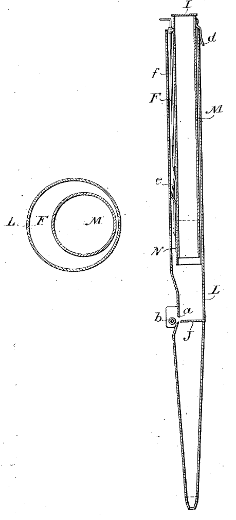
In 1910 William E Haskell of the Estey organ company in the USA was granted a patent for a novel means of deriving a suboctave tone from a half length pipe [1]. In the embodiment usually encountered today it consists of an open pipe into the top of which is inserted a narrower tube which Haskell called the 'complementary chamber'. The complementary chamber is stopped at the top and it can extend downwards nearly as far as the mouth of the main (open) pipe if so desired. In this configuration the pipe speaks almost, though not quite, an octave lower than the pitch of the main pipe alone. The arrangement is illustrated in Figure 2 which is a sketch taken from the patent specification.
Figure 2. Typical Haskell metal pipe
The diagram has not reproduced well since the original in the patent specification was not good either, though it shows the complementary chamber hanging within the main pipe. The small diagram to the left of the figure is a plan view of the pipe showing that the two cylinders can be arranged eccentrically if desired, though nowadays it is more usual to mount them coaxially. Figure 3 below is an expanded view of an eccentrically-mounted arrangement at the top of the main pipe, again taken from the patent, showing the tuning rod which is connected to a sliding sleeve (out of sight) at the bottom end of the complementary chamber.
Fig 3. Expanded view of the top of a Haskell pipe
So far, so good, but nothing new has yet been described beyond that which an ordinary half length stopped pipe would exhibit, namely a speaking pitch corresponding to an open pipe of about twice the length. However the big difference between a stopped pipe and a 'Haskelled' pipe is that all the harmonics required in the tone are present, unlike the stopped pipe with its weak even-numbered harmonics. Therefore the tone of a Haskell pipe is more satisfactory than that of a stopped pipe, so it does not need helpers to improve the tone.
It is fair to say that nobody really seems to know how Haskell pipes work (if they claim to, ask them to elaborate). The patent is silent on the matter, and one of the few attempts to understand them is a brief mathematical paper written way back in 1937
[2]. Having studied this in some depth I am afraid that I harbour considerable doubts about it. The author first derives an equation which, on the face of it, confirms what Haskell claimed in his patent in that the sum of the lengths of the two tubes (inner plus outer) equals the length of the equivalent open tube as far as pitch is concerned. But the trouble with maths is that equations can obscure, rather than clarify, the physics of what is going on. In this case we (well, me) would like to know how air pressure impulses travel up and down within the double-tubed Haskell resonator, so that we can compare it with the simpler situation of an ordinary organ pipe where such a picture is widely accepted, easily understood and useful
[3]. However the paper then goes on to compare the theoretical frequency predictions with experimental results from real Haskell pipes, claiming close agreement. Unfortunately, both when deriving the equations and in assessing the experimental results it skates rapidly over the problematical and awkward question of end corrections in what is a decidedly complex acoustic contrivance. The phenomenon of end correction remains ill-understood to this day even in ordinary flue pipes, and for those who are interested there is a detailed article on this site where I investigated it in detail
[4]. In 1937 these uncertainties would have been writ large, and certainly with a Haskell pipe, to the extent that I cannot accept as valid the experimental results presented so glibly in Jones's paper.
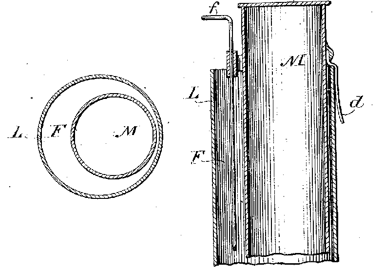
Figure 4. Haskell wood pipe
Figure 4 (the left hand sketch) shows an alternative configuration made of wood in which the main and complementary chambers are effectively separate pipes, one stopped and the other open. Thus one chamber is not inserted within the other as it was in Figure 2. You might now be able to see this arrangement as strikingly similar to that of the two separate helper pipes discussed earlier, the only (though major) difference being that the two pipes now share a common mouth. The two chambers in Figure 4 together emit all harmonics, the odd-numbered ones from the stopped chamber and the evens from the open one. This made me wonder whether Haskell was led to his invention by following a train of thought initiated by the helper idea, which was well known in his day. The composite pipe is tuned by a slide K at the bottom of the stopped pipe as shown by the right hand sketch in the figure (though as drawn it seems an impractical affair - how could one reach the clamping screws with a screwdriver once the pipe had been assembled?). Nevertheless this two-separate-pipes example provides some clues as to how a Haskell pipe works. It is pretty clear that the stopped pipe exerts strong control over pitch for several reasons. Firstly it is the stopped pipe which provides the fundamental frequency, since the open pipe on its own could only speak the octave above. Secondly it is the stopped tube in all configurations known to me which is adjusted when tuning the pipe. Thirdly, saying the same thing differently, adjusting the stopped pipe forces the frequency generated at the mouth built into the wall of the open pipe to vary. The acoustic mechanism whereby this happens remains to be discussed. Fourthly, this frequency defines the speaking pitch of the composite pipe, and it corresponds to that pitch which would be (approximately) obtained from the stopped pipe alone in Figure 4 if it had its own mouth.
When any type of Haskell pipe is speaking it must be voiced so that sufficient acoustic power in the mouth tone exists at all harmonics, both odd and even, to excite both pipes and cause them to jointly emit sound at all those frequencies. One therefore imagines that the necessary voicing adjustments at the mouth are critical to getting the relative proportions of odd to even harmonics acceptable, or even to get the pipe to speak at all. Since Haskell pipes are sometimes criticised for their excessively thin or stringy tone, perhaps this is the reason why - it might be difficult to arrive at a voicing condition where both pipes speak while their relative contributions to the acoustic power at the odd and even harmonic frequencies are in acceptable proportions. Unlike the helper arrangement with its separate pipes, it is not possible to voice both of the speaking chambers of a Haskell pipe independently, and this seems to me to be one of its drawbacks. In other words, voicing a Haskell pipe illustrates the art of achieving a compromise at best.
Nevertheless, we need to go a lot further to come up with a satisfactory physical description of how a Haskell pipe works, and this will now be done.
Figure 5.
Typical Haskell organ pipe configuration
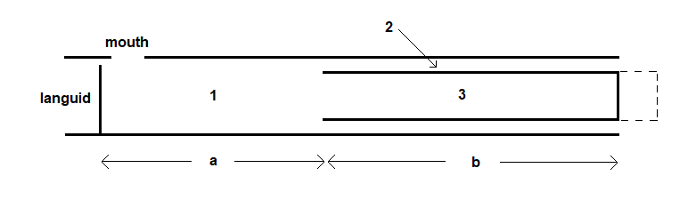
Figure 5 is a sketch of a typical Haskell pipe with coaxial resonators. It is based on a diagram which Jones used in his theoretical paper of 1937 [2] and the symbols here are the same. Thus the pipe is depicted in terms of three regions labelled 1, 2 and 3. The length of the open pipe (Haskell's 'main chamber') is a + b and that of the stopped pipe (the 'complementary chamber') is b. This representation might be convenient if you want to cross-refer to Jones's paper. However, there will be no mathematics here beyond a bit of the simplest arithmetic later on. Instead I shall attempt to paint a picture of what happens inside the pipe, in the same way as in my earlier article describing how ordinary closed and open flue pipes speak [3]. Unless you are familiar with how flue pipes work you might find it useful to open the latter article in another browser tab since I will be referring to it in what follows.
The acoustic processes inside a Haskell pipe will be described in terms of a number of successive time steps, in each of which the distance travelled by a sound wave is mentioned. When these distances are totalled up at the end of the discussion, the value thus obtained enables the frequency or pitch of the pipe to be calculated easily.
Step 1
Step 2
Step 3
The second thing which happens occurs at the same time, when the impulse in region 3 hits the closed top of the pipe. Again there is a sudden impedance mismatch which causes a reflection, but this time the reflected impulse remains with positive pressure - there is no phase change at the top of a stopped pipe. This also is explained in reference [3] (see the section dealing with stopped pipes).
Step 4
Step 5
When the impulses reach the top of their respective chambers, two different things happen simultaneously in the same way as before. Firstly, the positive pressure impulse in region 2 gets reflected back into the pipe, again becoming a partial vacuum because of the phase change at the open end. Secondly, when the impulse in region 3 hits the closed top of the pipe a reflection occurs, but the reflected impulse remains as a partial vacuum because there is no phase change at the top of a stopped pipe.
But something important has happened. The two impulses are now both partial vacuums, whereas previously they had opposite phases. Let's see what happens in the next step.
Step 6
Step 7
The total distance travelled by the impulses in the several steps above is as follows:
Step 1:
0
Frequency spectrum of a Haskell pipe
The emitted frequency spectrum of a Haskell pipe deserves consideration. Although the pipe can be made to sound about an octave below that which its length would suggest, its spectrum contains all harmonics, both odd and even. This contrasts with a stopped pipe which (like the Haskell) also sounds an octave lower than an open one of the same length, but here only the odd-numbered harmonics are emitted with appreciable strengths. Therefore a Haskell pipe combines the characteristics of both an open and a stopped pipe - like a stopped pipe it is much shorter than an equivalent open pipe would be, but like an open pipe it emits all harmonics. The explanation is that the resonating mechanism of a Haskell pipe is like that of an ordinary open one in that the oscillating air jet at the mouth is only synchronised once per cycle by an impulse returning down the pipe. We saw this above where a returning negative-pressure impulse sucked the jet into the pipe once per cycle. It can be shown that this mechanism results in all harmonics being generated, since each harmonic component in the jet's motion must also be synchronised once per cycle. In contrast, a stopped pipe synchronises the jet twice per cycle - it alternately pushes and pulls the jet into and out of the mouth at every half-cycle of the fundamental frequency - a phenomenon which can be shown to suppress the even harmonics in the jet's motion. Since this does not happen in a Haskell pipe, it therefore emits sound which includes all harmonics. This brief discussion concerning the mechanism of harmonic generation at the mouths of open and stopped pipes is expanded in reference [3] (see the 'tone quality or timbre' section).
There is, however, another mechanism at work in a Haskell pipe which does not appear in other types. In each of steps 3 and 5 above an impulse travelling in region 2 of the pipe reached the top of the annular space between the outer and inner tubes to meet the atmosphere. The phase of each impulse was the same (positive pressure in this example). Although the majority of the energy in the impulses will be reflected back into region 2 as described previously, a proportion of it will escape and propagate into the atmosphere to be heard at a distance from the pipe. Since there are two such impulses per cycle, this means that a Haskell pipe generates an enhanced second harmonic at an octave above the fundamental frequency of the pipe. It also means that other harmonics will probably be enhanced to some extent, depending on how 'sharp' the impulse is. If it is of short duration and with steeply rising and falling edges, it will generate more power at the higher harmonics than if it is a longer and 'smoother' pulse. The pulse shape will depend partly on how the voicer treated the mouth of the pipe as well as the pipe scale. Nevertheless, there will always be two pulses generated per cycle at the top of the pipe which will therefore enhance the acoustic power at the second harmonic, together with that at some others. Subjectively, the effect is likely to be similar to that obtained with a separate 'helper' pipe which is too loud. This phenomenon might explain why the tone of Haskell pipes is disliked by some, who have described it using various adjectives such as 'thin', 'stringy' or even 'gruff and unfriendly'. It illustrates a disadvantage of Haskell pipes, since trying to compensate for the effect through voicing adjustments at the single mouth is difficult if not impossible, whereas the power and tone quality of a separate pipe (which generates the even-numbered harmonics in a 'helper' system) can be readily controlled.
This prediction of second harmonic enhancement due to Haskelling was made before the necessary experiments were actually carried out on a Haskell pipe. However this has now been done and the prediction has been confirmed in a sequel article now on this site [5].
Two methods for deriving real suboctave tones from half length pipes while retaining all the even and odd-numbered harmonics have been discussed. The use of separate open helpers to provide the even harmonics, together with stopped pipes which supply mainly the odds, offers considerable voicing flexibility to the extent that it can be impossible to detect that the system is in use. The technique was illustrated in terms of the harmonic spectra of both constituent pipes.
1.
US patent 965896, 2 August 1910.
5.
"Experiments on a Haskell
organ pipe", an article on this website, C E Pykett 2022
|