


|
|
|
Experiments on a Haskell organ pipe
Colin Pykett
Posted:10
October 2022
Abstract. This article is a sequel to an earlier one [1] which described, probably for the first time, the physics of Haskell pipes without recourse to mathematics. Some predictions were also made about certain features which might be seen in the acoustic spectra of Haskell pipes before they had actually been observed. Consequently the work described here was undertaken to investigate these predictions experimentally. In particular it was suggested in the earlier work that a Haskell pipe would exhibit a strong second harmonic, and this has now been confirmed. It is shown here that the SPL of the second harmonic increased by at least 10 dB relative to the fundamental when a Gamba pipe was Haskelled, consequently this supports the theory of operation of the Haskell pipe put forward in the earlier article. It is also shown how the fundamental frequency of a Haskell pipe can be predicted easily to better than 2% of its measured value.
Although the acoustic spectra of an extensive range of ordinary organ pipes have now been published and discussed widely for nearly a century, none relate to Haskell pipes as far as is known. The differences between Haskelled and non-Haskelled spectra presented here are therefore believed to be unique in the public domain literature. In this article they are related to criticisms of the 'Haskelled sound' which have long been articulated within the organ building community.
Contents (click on the headings below to access the desired section)
Introduction
In a previous article [1] I described William Haskell's method for obtaining a much lower pitch (frequency) from an organ pipe than its physical length suggests. A stopped pipe does the same thing but it also suppresses the even-numbered harmonics in its tone, rendering it unsuitable for some purposes. In contrast, a Haskell pipe generates a complete retinue of both the even and odd harmonics. The article presented a theory of how Haskell pipes work, since it is fair to say that nobody really seems to have understood them ever since the original patent appeared in 1910 [2]. Since predictions were also made in the article about some artefacts which might be observed in the acoustic spectra of Haskell pipes, the work described here was undertaken to investigate these prophecies experimentally. They were confirmed, thereby also validating the theory on which they were based.
Following Haskell's terminology in his patent specification, the two tubes which constitute a Haskell organ pipe are referred to here as the 'main' (outer) pipe and the 'complementary' (inner) pipe.
To restrict the length of this article, repetition of material in the earlier one is minimal. Therefore you might want to open the previous article in another browser tab to make cross-referencing easier.
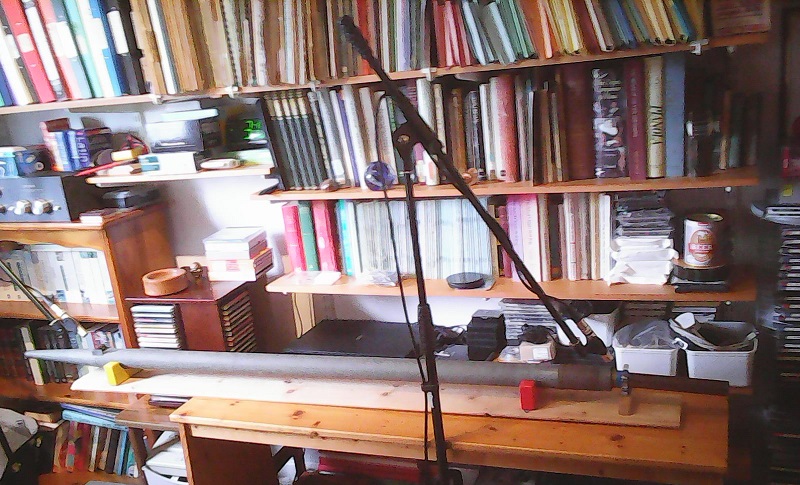
A test rig was made which cradled the main (outer) pipe horizontally and it also allowed the relative position of the complementary (inner) pipe to be adjusted easily. Two high quality electret microphones were positioned close to the mouth and top of the outer pipe but upstream of the air flow. This avoided the signals being dominated by low frequency noise of high amplitude due to air turbulence enveloping the microphone capsules, a particular problem with electrets since their response is maintained down to very low infrasonic frequencies. The microphone signals were recorded into a wave editor (WaveLab) running on a laptop computer. The general arrangement of these items (excluding the computer) is shown in Figure 1.
Figure 1. Haskell experiments - general arrangement of the test rig
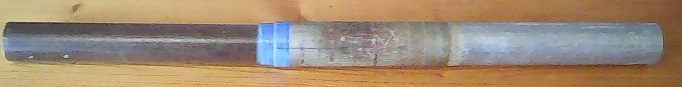
The complementary (inner) pipe assembly is shown in Figure 2. The pipe itself was of thin-walled metal tubing with a tight-fitting stopper made from a length of wooden rod. To facilitate adjustments, the rod was far longer than would have been required in an actual Haskell pipe. The joint between the pipe and the stopper was made completely airtight using adhesive tape.
Figure 2. Complementary pipe assembly
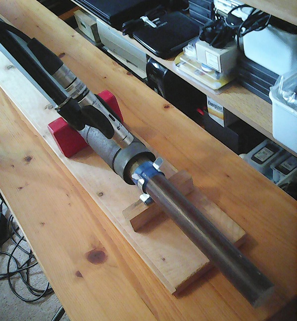
Figure 3. The complementary pipe in situ inside the main pipe
Dimensions of the test rig and its components which were relevant to the experiments are listed below. Two in particular were deemed important in view of what Haskell wrote in his patent. The first was that the cross-sectional area of the annular space between the inner and outer pipes should be the same as that of the inner pipe. Thus the internal areas of the two pipes should be related by a factor of two. Achieving this was constrained in these experiments by the diameters of the two pipes which were available, but a reasonably close match was obtained (the areas were actually related by a factor of 2.4). The wall thickness of the inner pipe was ignored here. The second point was that the top of the inner pipe (the point where the air column met the stopper) had to project by a prescribed amount beyond the top of the outer pipe (as specified in the list below). In fact, experiments showed that this dimension was not as critical as the patent implies, though it was adhered to as closely as possible.
One way to establish whether the Haskell pipe was working as intended was to calculate (i.e. predict) the fundamental frequency or musical pitch of the note it should emit, and compare it with that actually obtained. The following analysis uses only simple arithmetic, in which some results are rounded to avoid propagating large numbers with needless precision.
Starting with the main pipe alone, its frequency was measured from the dual-channel microphone recording as 120.2 Hz using the facilities of a wave editor (WaveLab). This corresponded approximately to the pitch of bottom B on an 8 foot stop. Since wavelength equals sound speed divided by frequency, this means that the wavelength of the sound was 343000/120.2 or 2854 mm, where the speed of sound was taken as 343 metres per second. Because an open flue pipe (including its end corrections at the top and mouth) is exactly one half-wavelength long [3], the effective length of the pipe was therefore 2854/2 mm or 1427 mm. The adjective 'effective' means that the end corrections are conveniently included in this figure as we have used the frequency at which the pipe actually spoke, thus we do not need to estimate values for them. Consequently the effective length is somewhat longer than the internal length of the pipe (1293 mm), as would be expected.
When the pipe had its complementary tube inserted it was speaking in Haskell mode, and we want to predict what its speaking frequency will be. Here we need first to estimate a value for the end correction at the open end of the complementary tube situated inside the outer pipe. The usual value of 0.3D (D is the diameter) is a reasonable approximation to the end correction of a cylindrical pipe, thus the correction will be 0.3 x 32 mm which equals 9.6 mm. This gives a total value for the effective length of the complementary tube as 303 + 9.6 mm since its internal length measured up to the stopper was 303 mm. Since a Haskell pipe speaks as an open pipe with a combined length of both tubes, we therefore get a total effective length of 303 + 9.6 + 1427 mm which equals 1740 mm.
Because the effective length of any open pipe represents a half-wavelength of the emitted sound [3], we get a value of 1740 x 2 or 3480 mm for the wavelength. And since frequency equals sound speed (343 metres per second) divided by wavelength, the speaking frequency of the Haskell pipe is therefore predicted to be 343000/3480 Hz or 98.6 Hz. This is very close to the actual frequency of the experimental Haskell pipe, which had been measured in the wave editor as 100.0 Hz (approximately the pitch of bottom G# on an 8 foot stop). Therefore the pipe was certainly behaving as a Haskell pipe should, and the foregoing discussion has shown that it was straightforward to predict its frequency to better than 2%.
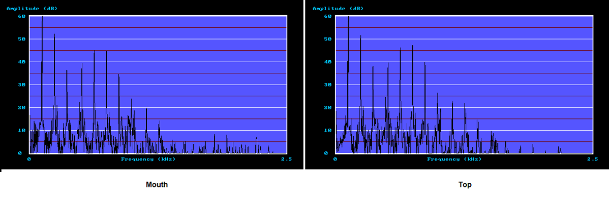
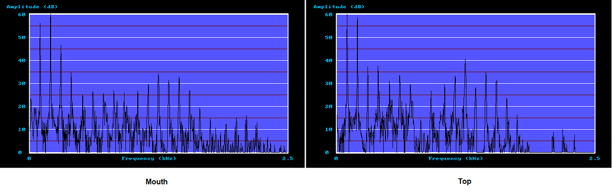
It is of interest to examine the frequency spectra of the pipe both when speaking alone and when Haskelled, since some predictions were made in the earlier article [1] (perhaps rashly) about the likely harmonic content of a Haskell pipe before the data from these experiments had become available. Moreover, to the best of my knowledge the acoustic spectrum of a Haskell pipe has not appeared previously in the public domain literature. Thus Figure 4 shows the spectra of the two microphone signals from the mouth and top of the main pipe when speaking alone.
Figure 4. Spectra at the mouth and top of the main pipe when speaking alone
The vertical axes display sound pressure level (SPL) as a function of frequency, represented in decibels, the dynamic range of 60 dB corresponding to an SPL ratio of 1000 to 1. A greater value would have added nothing useful since it is obvious from the plots that lower-level signals would have been visually submerged within the noise floor (the noise having been contributed mainly by air turbulence at the languid and pipe mouth). Both spectra were normalised independently to the amplitude of the strongest harmonic to which was assigned the arbitrary value of 60 dB, therefore each plot shows relative rather than absolute SPL values, and moreover there is no relativity between them. The normalisation is of no consequence for the purposes of this article.
Several features are of note. Firstly, the two spectra are remarkably similar both in overall shape and in terms of the relative numerical amplitudes of their constituent harmonics. Secondly, both spectra contain about the same number of harmonics (10 or 11). Thirdly, the fundamental (first harmonic) is the largest in both cases. Fourthly, a pronounced formant-like hump near 720 Hz is visible, centred around the sixth harmonic. The fact that the two spectra were so similar gave some confidence that room effects were not a major factor when recording the signals, otherwise one would have expected to see more obvious visible differences between them. Significant room effects are usually noticeable in a spectrum and very sensitive to microphone position.
Comparing these results with those for the pipe when Haskelled, the two corresponding spectra are shown below in Figure 5.
Figure 5. Spectra at the mouth and top of the pipe when Haskelled
These differences could be related to a marked disparity between the timbre or tone colour of the pipe when speaking in the two modes (i.e. alone and when Haskelled). In the former case it sounded much as one might expect of a well-scaled and expertly voiced Gamba pipe of this intermediate pitch, having an attractive resonant purr which was probably related to the pronounced formant band around 720 Hz. But when speaking in Haskell mode its tone became scratchy and uninteresting. Anything akin to a Gamba sound of reasonable pedigree had vanished. There was no longer any character to it - the weaker fundamental had become difficult to distinguish against the background of a very strong second harmonic plus the combined power of many others, and any helpful effect of the emasculated formant band (now of lower amplitude and at a much higher frequency) was impossible to discern. There was no doubt in my mind that one effect of Haskelling this pipe, and probably any Haskell pipe, was to encourage it to generate far too many harmonics. It is conceivable that voicing adjustments could have improved matters. Raising the upper lip, thereby increasing the cut-up of the mouth, might have been beneficial as this would have reduced the acoustic power at the higher harmonics. However I was unwilling to attempt this as it would have been an irreversible mutilation of an otherwise serviceable pipe.
These criticisms of the 'Haskell sound' are of a piece with those often articulated elsewhere. The late Stephen Bicknell probably had as refined an ear for these matters as anyone, and he opined that "Haskell basses are rather gruff and unfriendly in tone. They are really too coarse to be used in the 8ft octave (where a helper is actually more musical ... )" [4]. The pipe used here would indeed find its place in the 8ft octave, so his remarks pretty much chime with mine. Since criticisms such as these are fairly widespread across the organ building community it is probable that little improvement can be effected through voicing, notwithstanding my suggestion above concerning cut-up. When all is said and done a Haskell pipe consists of two physically separate tubes, tuned to different frequencies but sharing a common mouth, and generating yet a third frequency. Seen in these terms it is, frankly, a somewhat bizarre contrivance and it would not be surprising if the best that can be achieved by a voicer is some sort of compromise between getting the pipe to speak at all and it speaking with an unappealing tone quality. However, in fairness Bicknell did qualify his opinion by averring that "the most effective use of the Haskell technique I know of is in turning an old 16' open wood into a very successful 32' rank", and it is in this situation where its attributes of much smaller size and (possibly) lower cost come to the fore most strongly. Perhaps these are so attractive to the organ builder and customer that they overcome reservations about tone quality. But if these should arise it is unfortunately too late since the organ will already have been built and paid for, leaving the owner with no option but to advertise a dubious virtue out of necessity. However, on the positive side, there will be many situations where a 32 foot stop (other than a fake resultant bass) could not have been installed at all without resorting either to a stopped rank or to Haskelling, despite the different limitations of both approaches.
In the previous article I hazarded an educated guess that a Haskell pipe would exhibit a strong second harmonic [1]. At the time this was purely a prediction made on the basis of the novel theory of operation which I had just outlined, and it was made before I had seen the spectra presented here in Figures 4 and 5. But since they show unequivocally that the prediction was correct, they also suggest that the theory itself is sound.
This article is a sequel to an earlier one [1] which predicted certain features which might be observed in the acoustic spectra of Haskell pipes before they had been seen. Consequently the work described here was undertaken to investigate these predictions experimentally. In particular it was suggested that a Haskell pipe would have a strong second harmonic, and this has now been confirmed. It has been shown here that the SPL of the second harmonic increased by at least 10 dB relative to the fundamental when a Gamba pipe was Haskelled, consequently this supports the theory of operation of a Haskell pipe put forward in the earlier article. It has also been shown that the fundamental frequency of a Haskell pipe can be predicted easily to better than 2% of its measured value.
Although the acoustic spectra of ordinary organ pipes have been published and discussed widely over nearly a century, none relate to Haskell pipes as far as is known. The differences between Haskelled and non-Haskelled spectra presented here are therefore believed to be unique in the public domain literature. In this article they have been related to the fairly widespread criticisms of the 'Haskelled sound' which have long been articulated within the organ building community.
I am grateful to my friend Mr Paul Minchinton for having provided the Gamba pipe used in these experiments.
1. "Helpers and Haskells", an article on this website, C E Pykett 2022
2. US patent 965896, 2 August 1910
3. "How the flue pipe speaks", an article on this website, C E Pykett 2001
4. "Harmonics and cheats", Stephen Bicknell, https://www.stephenbicknell.org/3.6.01.php (accessed 9 October 2022)
|