


|
|
|
Equalising Loudspeaker Sensitivities
by Colin Pykett
"when you cannot express it in numbers, your knowledge is of a meagre and unsatisfactory kind" Lord Kelvin
Posted: 17 September 2012 Last revised: 19 May 2013 Copyright © C E Pykett 2012
Abstract. This article presents some work on loudspeakers to illustrate how they radiate sound in rooms and how they can be improved. It describes a considerable amount of experimentation, construction, practical measurement and how the results were analysed. The article is aimed mainly at the electronic organ application, but it is equally relevant to high quality audio more generally. The main intention was to equalise the sensitivities of tweeters and woofers but several other aspects of loudspeaker design are visited, including multipath propagation in rooms, practical means for performing near-anechoic measurements, the choice of test signals and matched attenuators. A thesis of the article is that room effects are so dominant that it is pointless getting too hung up about some details of loudspeaker design and performance, such as the minutiae of crossovers and baffle effects. Unfortunately one rarely comes across actual measurements such as those presented here to demonstrate this point. The consequence is that only major shortcomings can be detected by the ear in a real room, such as that which initiated this work in the first place to do with the mismatched sensitivities of disparate drive units.
Contents (click on the headings below to access the desired section)
In-room Loudspeaker Measurements
Appendix 1 - L-pad attenuator design
This article presents some work on loudspeakers to illustrate how they radiate sound in rooms and how they can be improved. It describes a considerable amount of experimentation, construction, practical measurement and how the results were analysed. The article is aimed mainly at the electronic organ application, but it is equally relevant to high quality audio more generally.
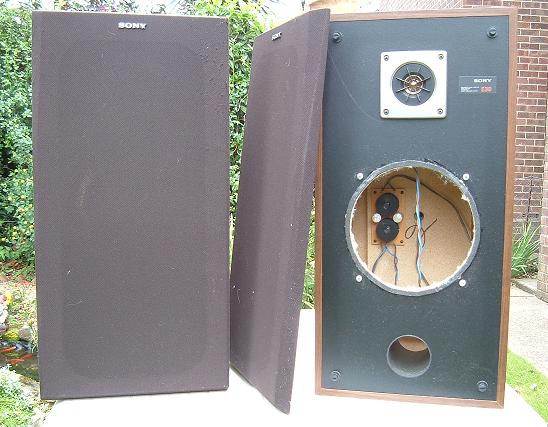
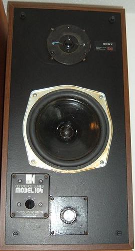
It all started when I came by an old pair of Sony SS-E30 loudspeakers (Figure 1).
Figure 1. Sony speaker cabinets
The drive units they contained (an 8 inch woofer and a dome tweeter) were cheap and nasty, so they rapidly found new homes via eBay. However I was looking for some reasonably well made speaker cabinets for experimental purposes because making one's own is far too difficult and time consuming, and the Sony boxes fitted the bill very well in this regard. They were required to house some high quality KEF drivers (B200/SP1014 woofers and T27/SP1032 tweeters) which I had been fortunate to find as new old stock. These were used in various KEF speaker systems of the day such as their respectable 'Chorale' product. I also had a spare pair of KEF high-end crossover networks as used in their flagship 'Reference 104' loudspeakers. And because the Sony cabinets were well matched to the enclosure volume required by the SP1014 when used in a sealed box, the whole project seemed to be coming together nicely.
However the revamped speakers with the new drive units were so tiring to listen to that I found them almost intolerable over extended periods. Bass response was subjectively good down to about 40 Hz (bottom D# at 16 foot pitch on the organ), much as one would have expected from an enclosure of this size with the SP1014 drive unit. But there seemed to be some high frequencies which almost hurt the ears, and treble response generally was just far too 'bright'. It did not take long for me to suspect that the woofers and tweeters were not well matched in sensitivity, with the tweeters being more sensitive than the woofers. This is a common problem with loudspeakers, including some expensive ones. But although the problem was simply stated, if indeed this was the problem, doing something about it was quite another matter. The first step had to be to estimate the disparity in sensitivities, and the second was how to equalise them.
This issue is just as important for electronic organ applications as any other because a conventional multiple-driver loudspeaker is required for most of their audio channels if the full harmonic spectrum of each note is to be handled. For instance, when playing middle C on a stop with many harmonics such as an 8 foot reed or string, those after the 12th will often be handled by a tweeter because they will lie beyond 3 kHz or so, which is around the maximum applied to a typical medium frequency drive unit. In this situation it is therefore essential to ensure that the sensitivities of the drive units are well matched otherwise the intended timbre or tone quality of the note will be corrupted. Also, for any application with multiple drivers, it is immaterial whether the conventional arrangement of a single amplifier feeding a crossover network is used or whether bi-amping is employed in which each driver is powered independently. In both cases it is necessary to equalise the acoustic outputs of both drivers, which means that one has to know when equality has been achieved. It is scarcely necessary to add that subjective listening tests are hopelessly inadequate when trying to estimate discrepancies in sensitivity.
This is the subject of the article, and the technical journey I embarked on will now be described. It includes the choice of test signals, how to interpret in-room measurements, whether free field measurements are useful and how to perform them, crossover networks and matched attenuators. Regarding the latter, complete details are given for designing L-pad attenuators because much of what one finds on the Internet is wrong. In passing the article also contemplates issues like whether crossovers, baffle effects and other aspects with which some loudspeaker designers seem to be besotted are really all that important when set against what real rooms do to sounds arising within them.
A key aspect of this work was to estimate as accurately as possible the apparent discrepancy in sensitivity between the tweeters and the woofers. An obvious approach was to measure the frequency response of the loudspeaker and see whether there was a significant change in acoustic output either side of the crossover frequency, as measured using a microphone. This was essentially the approach I pursued, but it was far easier said than done. Firstly it was necessary to decide which type of test signal to use. There are two types of wideband test signal - a swept frequency sinusoidal tone or wideband noise. Swept tones are often employed, but they can lead to difficulties when interpreting the results. For instance, if the tone is swept too quickly the acoustic response of the room can mask the effects being observed. In simple terms this means the tone needs to spend enough time at each frequency across the spectrum to enable the reverberation in the room to stabilise. This applies to all rooms no matter how small unless the room is anechoic, which no ordinary room is. Thus it can be a time consuming business because it is easily possible to end up with a sweep time occupying minutes rather than seconds.
The other type of test signal uses random noise, usually pink or white noise, which contains all frequencies simultaneously. However it is then desirable, if not essential, to average the results so that the statistical fluctuations inseparable from the noise signal can be suppressed. Fortunately the averaging process in this case takes only a few seconds at most because it is applied simultaneously to all frequencies. This was the approach used here.
White noise has equal power in a given bandwidth across the frequency spectrum of interest. Thus if we take a bandwidth of 10 Hz, say, we get the same signal power wherever we put that band in the audio spectrum. Therefore its main disadvantage is that the power in each octave varies radically, because an octave in the bass register between 30 and 60 Hz, say, represents a bandwidth of only 30 Hz whereas an octave between 4 and 8 kHz represents a bandwidth of 4 kHz. This means the treble octave contains 133 times more noise power (more than 21 dB) than the bass octave. When doing practical loudspeaker measurements this can result in the woofer being comparatively underdriven in terms of the total power applied to it, whereas the tweeter might be overdriven to the extent it could be damaged. Pink noise solves this problem because its power per unit bandwidth is not a constant as for white noise, but is inversely proportional to frequency. This means pink noise contains more energy at bass frequencies, and this can easily be heard when listening to the two types of noise. Thus one does not need as much system gain to get sufficient bass power when using pink noise, with the result there is less risk of damaging the tweeter.
Either 'colour' of noise could have been used here, but I prefer to use white noise whenever possible. This is because it produces a nice flat horizontal line on a frequency response type of display (neglecting the random fluctuations), whereas pink noise can produce a sloping or curved line depending on whether the display uses linear or logarithmic axes. As it is generally easier to spot variations from a flat line than a curved one when trying to interpret the results, I opted for white noise in these tests.
The amplitude (voltage) versus frequency spectrum of computer-generated white noise across a frequency band from almost zero to 12 kHz is shown in Figure 2.
Figure 2. White noise frequency spectrum (not averaged)
Several points are worth noting. Firstly, although the mean spectrum is indeed flat there are considerable excursions about that mean, some of which reach nearly -30 dB. More will be said about this presently when we discuss how to reduce them. For now, note that the apparently asymmetrical deviations from the mean are merely due to the use of a decibel scale - the peak negative excursions up to -30 dB are balanced by positive ones of up to +6 dB in round figures, which is as expected for white noise and what we see in the spectrum. If a linear scale had been used the positive and negative excursions would have appeared similarly distributed in amplitude about the mean level [4].
The second point concerns the mean spectrum level itself, which is below -50 dB in this example. At first sight this might suggest that I was using an excessively weak signal. After all, zero dB on this display corresponds to the maximum amplitude of a 16 bit signal, so -50 dB means the average level of the spectrum amplitude values was around 316 times lower than this maximum. So why did I not crank up the gain a bit more? In fact this would not have been possible. The wideband signal constituting the white noise was the sum of a large number of elementary sine waves with random amplitudes and phases at all frequencies across the spectrum, and this was necessarily adjusted in amplitude so that its peaks did not saturate the spectrum analysis program (i.e. so that they did not exceed 16 bits). But having made that adjustment, it meant that the amplitude of each elementary sine wave was then much lower than the amplitude of all of them when added together. Therefore, whenever similar spectrum plots occur throughout this article, they will all be of much the same mean level. Bear in mind this does not mean that the results represent measurements of low signal to noise ratio.
A third observation takes us back to the 'grassy' nature of the plot. Such excessively grainy data are not really much use when trying to spot things like differences in level between the outputs from a woofer and a tweeter. Fortunately we can improve things considerably by noting that successive spectra (successive snapshots if you like) computed from a continuous white noise signal are completely different. Although the mean level will stay the same, the level at any one frequency will fluctuate considerably from one spectrum to the next. It is impossible to predict what the next spectrum level will be at a given frequency other than in a broad statistical sense, because white noise is generated by a random process. Thus by averaging successive spectra, the fluctuations seen in Figure 2 will be dramatically reduced, and this is shown in Figure 3.
Figure 3. White noise frequency spectrum (averaged over 35 samples)
This picture was produced using 35 averaged spectra, which took just a few seconds to compute. The most significant improvements occur for the first few averages and as many as 35 is possibly gilding the lily. However this figure was used throughout this work, partly because it is fascinating to observe the changes as each plot appears in real time. It is important to compute the averages using the linear spectrum values before conversion to decibels for plotting. One must not average the logarithmic quantities because of their asymmetric distribution about the mean as mentioned above, and I suspect the originators of some commercial acoustics analysis packages (for which one is expected to pay good money) might have fallen into this trap on the basis of the strange and wholly erroneous averaged results they produce. Averaging must not perturb the mean value, only the fluctuations either side of it [4].
The fourth feature is that a linear rather than logarithmic frequency scale was used. This was because I was mainly interested in the tweeter response above the crossover frequency, so I wanted this to occupy a good proportion of the horizontal display. A logarithmic scale would have expanded the woofer response, which was of less interest for reasons which will become clearer later in the article.
The fifth aspect concerns the meaning of the spectrum values in decibels when loudspeaker frequency responses were measured as described in a moment. Briefly, this was done by applying white noise to the speaker, picking up the resulting acoustic signal with a microphone and then spectrum-analysing it. The capacitor microphone used gave an output voltage proportional to sound pressure level (SPL). SPL is similar to voltage in that both are entities which are capable of doing work and thus generating power - they can be considered as amplitudes or forces if you like, but they are not measurements of the power itself. Therefore the SPL frequency spectra in this article - computed from the microphone voltages - are plotted on a decibel scale in which 6 dB equals a factor of two, 20 dB a factor of ten, etc. To convert these to power the factors have to be squared because electrical power is proportional to the square of voltage, and acoustic power is proportional to the square of SPL. Thus for power, 6 dB represents a ratio of 4, 20 dB a factor of 100, etc. Therefore the spectrum simultaneously represents acoustic amplitude (SPL) and acoustic power depending on how you want to use the dB values. Although this might sound confusing, you have to be careful how you use decibels otherwise major errors can be introduced. Note also that the SPL levels are not absolute pressure measurements; they are relative to an arbitrary datum representing the maximum value of a 16 bit voltage waveform. This was assigned a level of 0 dB.
The sixth and final aspect of these plots is that they were generated using spectrum analysis and display programs which I wrote myself. This was because I could find no other product which offered the flexibility and features I wanted.
Although the ultimate intention was to make measurements on loudspeakers with the aim of improving them, I first looked at the frequency response of some good headphones. This was because headphones, unlike loudspeakers, do not use multiple transducers with crossover networks. Instead they use single wideband transducers which are not called upon to radiate much acoustic power. Therefore issues of conversion efficiency (electrical to acoustic) do not arise with phones, and this makes it easier to design suitable transducers which will work well across the entire audio spectrum. Thus I was interested to see how flat or otherwise their measured frequency response was, mainly because it would help to confirm whether the microphone I was intending to use had a flat enough response also.
It would have been a waste of time using poor units, and I used Sennheiser HD650 audiophile headphones. An electret capacitor microphone of reasonable quality, advertised with a nominally flat frequency response (but aren't they all?), was placed about 2.5 cm from each earpiece in turn. Fortunately this type of microphone usually does have a reasonably flat response, at least flat enough for the purposes of this article, but this test was intended to confirm it. Each earpiece, one at a time, was supplied with white noise at a level which had previously been adjusted to be comfortable to listen to. Results are in Figure 4, averaged over 35 spectrum estimates as described above..
Figure 4. Measured Sennheiser HD650 headphone frequency response
It was assumed that headphones of this quality would have had a tolerably flat frequency response over much of the audio spectrum, particularly as this product is still (2012) being advertised as having matched earpieces. If we cannot assume this, we might as well pack up and go home. Moreover, as the two earpieces were tested with one and the same microphone, one could reasonably presume that significant and similar peaks and troughs belonging to the microphone would have been visible in both spectra were its response not substantially flat. The result for the right hand earpiece is flat within a little over ± 3 dB, which is pretty good considering the plot represents the combined effects of a radiator (the earpiece) and a receiver (the microphone), neither of whose characteristics were known independently. Results for the left hand earpiece were not quite as good, lying within ± 5 dB. The measurements also suggest a dip in the mid-frequency region of both plots which therefore might have been a property of the microphone, but without calibrating it (which is unfeasibly difficult and expensive) it is not possible to draw more definite conclusions. Therefore these dips and the other differences between the plots could just as easily have been properties of the phones. As it is, the variations probably reflect relatively small differences between the two earpieces at least as much as the microphone characteristics. Similar, though not identical, results were obtained from similar runs in which the phones and microphone were moved to different positions. It was concluded that the microphone did not seem to be doing anything gross to the sounds presented to it, and that was the object of the exercise.
And now, dear reader, let me emphasise that this is pretty much as good as it gets in audio, as you will now see when we try to measure the response of a loudspeaker in a room. The relatively minor variations observed for the headphones then start to look like sheer perfection. If only we could get our loudspeakers to perform like this. Ugh. Get a cup of coffee first before you read on.
In-room Loudspeaker Measurements
It is one of the most unfortunate constraints in audio that we have to listen to loudspeakers in rooms. The human auditory system did not evolve to cope with the vagaries of room acoustics because our distant ancestors spent most of their time outside in nearly free field conditions, thus the way we subjectively perceive sound in rooms has to be learnt and laid down in our brains during early life. Consequently everyone perceives sound differently and has different opinions on it. For this reason there cannot, by definition, be an objective consensus on whether a particular loudspeaker is 'good' or not when we listen to it in a room. The only fixed star in this subjective firmament remains the physics of sound propagation in rooms, but unfortunately this is theoretically complicated. Not only that, but the effects are expensive, difficult and time consuming to measure experimentally. This seems to be a tacit excuse for ignoring the problems more often than not, to the extent that more than a few pundits seem to have little knowledge and first hand experience of room acoustics judged on the basis of what they write. Therefore we need to understand a little of what rooms do to sounds radiated from loudspeakers. Consequently one of the speakers was supplied with white noise in an ordinary room and its acoustic signal picked up with the same microphone used for the headphone experiments, placed 1 metre on-axis from the cabinet. The frequency response, averaged over 35 spectra as before, is shown in Figure 5.
Figure 5. Loudspeaker frequency response measured in a room
Wait a minute, I hear you cry - this response could not possibly have been averaged because the graph looks pretty much like the ragged one in Figure 2, which showed a non-averaged noise spectrum. Unfortunately you would be wrong if you held this view. Averaging only reduces random fluctuations which are different between one spectrum and the next. It does nothing to artefacts which are systematic, that is, those which are constant properties of the system under test. In this case these artefacts are room effects which are the same from one spectrum to the next, so they do not get averaged out. The pronounced variations in this response arose largely because of multipath propagation in the room. This is due to the direct sound from the loudspeaker drive units interfering at the microphone with sound reflected from the walls, floor, ceiling and furniture. If the microphone was to be moved relative to the speaker, even ever so slightly, the detail of the picture would change. It would completely change if the microphone was moved by a larger amount, with all the observed peaks and troughs being replaced with a new set. The fluctuations arise from the amplitudes and phases of all the reflected and scattered waves at a given frequency reaching the microphone simultaneously, as does the direct wave from the loudspeaker. They all add together to produce a single summed sine wave at this frequency, which will usually have an amplitude and phase considerably different from those at neighbouring frequencies. It is only the amplitude variations which give rise to the grassy nature of the display because phase information is discarded when computing the frequency response [5].
But it is possible to extract some useful information nevertheless. Notice the 'slow' periodic variations starting near the centre of the response and extending to the high frequency limit. Their peaks (and troughs) are separated by about 1500 Hz, and it is probable that the proximity of the tweeter to a dominant reflector in the room gave rise to them. As the speaker had been placed on a shelf during this test which put the tweeter about 25 cm from a hard plaster ceiling, simple geometry confirms that this was probably the case. Figure 6 is a sketch of the setup.
Figure 6. Multipath propagation in a room: speaker - ceiling interaction
The microphone at A is shown receiving the direct signal from the tweeter at C plus a wave reflected off the ceiling at B. The path difference between the direct wave propagating along the path AC and the reflected wave along the path BC + AB can be found using straightforward geometry, and it was 22.3 cm. The dimensions of the setup sketched in Figure 6 are given at note [2] from which this figure can be confirmed. When the two waves arrive at the microphone in phase (i.e. with a phase shift of zero or multiples of 360 degrees) there will be an enhancement of the signal level, and when in antiphase (phase shifts of 180, 540 (= 360 + 180), 900 (= 360 x 2 + 180), etc degrees) there will be a reduction. Enhancements will therefore occur for frequencies whose wavelengths are 22.3/N where N is an integer (N = 1, 2, 3, etc). Thus the first such peak should occur at a frequency of just over 1500 Hz, because frequency equals the speed of sound (33528 cm per second) divided by wavelength. However this frequency was not radiated by the tweeter but by the woofer owing to the action of the crossover network, and as the woofer was not at the same position as the tweeter the geometry of the situation was different. Therefore we must ignore this frequency. But successively higher frequency peaks will occur at multiples of about 1500 Hz, and this is precisely what the response shows when the periodic ripples start to develop in the high frequency region handled by the tweeter. Hence the ripples were largely due to the proximity of the ceiling to the tweeter.
These pronounced ripples with amplitudes approaching 30 dB in the frequency response might be considered undesirable, and this has probably led to the widely held view that loudspeakers should not be placed too close to the ceiling and walls. The distance between tweeter and ceiling can be increased by placing the speaker cabinet upside down if it must sit on a high shelf, but this does not solve the problem. It only replaces it with another which is worse. A greater tweeter-ceiling distance means that the path difference (AB + BC - AC) in Figure 6 gets larger, and this means that the separation of the frequency response ripples gets smaller. This factor is responsible for many rooms imposing a sort of 'drainpipe' sound on music, because pipes have a comb-shaped frequency response similar to that which can be generated by multipath propagation in rooms. Ripples will always occur to some extent if there is multipath, and there always is, and it is aurally better to have a few of them well separated in frequency as in Figure 5 rather than many which are closer together. This reduces the subjective 'drainpipe' effect. Therefore the speakers should be placed as close as possible to dominant reflecting surfaces. Note that this advice runs exactly counter to much accepted wisdom governing loudspeaker placement relative to walls and ceilings. For interest, an example of a more pronounced 'drainpipe' effect measured in another room with a different though high quality loudspeaker (a KEF Reference 104aB) is shown in Figure 7. Here the tweeter frequency region is dominated by many more, relatively closely spaced, ripples than in the previous example (Figure 5).
Figure 7. Illustrating the 'drainpipe' effect due to pronounced, though not untypical, multipath propagation in a room
Having seen and assessed these examples of typical room responses we might consider rethinking our position on loudspeakers. One often comes across derogatory phrases like "with such-and-such a loudspeaker you are mainly hearing the box", but a better one might be that "with ALL loudspeakers you are mainly hearing the room". The results also call into question the desirability of using 'wet' recordings of organ pipe sounds (i.e. those made with the deliberate aim of retaining room effects) in digital organs or virtual pipe organs using sampled sound synthesis. It is impossible to modify the resultant sounds when the organ is played because they were fixed once and for all at the time the samples were taken, therefore the sounds made by the actual pipes were irretrievably lost. Unless one really does enjoy 'listening to the room' as it sounded at an arbitrarily-chosen and fixed position rather than to the sounds of the pipes, it seems to me that using wet samples is exactly the wrong thing to do. These matters are addressed in detail in another article on this website. [3].
Returning to the loudspeakers which are the subject of this article, another feature of the frequency response shown in Figure 5 is that its overall trend, neglecting the peaks and troughs, increases with frequency. This can be seen by placing a ruler across the top of all the spectrum peaks, when an increase of about 6 dB across the spectrum as a whole takes place. This is a significant amount in audio terms. The subjective loudness of the high frequencies relative to the low ones is related to the total power radiated by the tweeter compared to that radiated by the woofer. Total power is proportional to the integral of the frequency response across the corresponding frequency range. It corresponds to the area of the approximate rectangle defined by the response curve itself and its height above zero. Therefore an increase of only a few dB in spectrum level will increase the rectangle area, and hence the radiated audio power, significantly because the increase affects all frequencies in a relatively broad band. This is why it is so important to equalise the sensitivities of the tweeter and the woofer - the adjustment is critical if one is to get it right.
As the spectrum level increased with frequency in this case, it confirmed that the tweeter was probably radiating too much power and that it was therefore more sensitive than the woofer. This confirmed my unsatisfactory subjective impressions when listening to this loudspeaker. How to solve this problem will be described presently.
But first let us play a new game I have invented. It is called "Spot the Crossover Frequency". Can you see the crossover frequency in the frequency response of Figure 5? I thought not. Although I could be really mean and tease you by not divulging it, it is at 3 kHz. This is a quarter of the way from the left hand side of the picture, which might or might not coincide with one of the many minor excursions in this frequency response. Many people apparently believe that a crossover notch (or blip, the difference depending on how the tweeter is phased relative to the woofer) is always obvious in a frequency response plot. But in this case it does not exactly jump out at you from the page. So should we actually worry so much about crossovers as most of us seem to do? Rather, should we judge them against the context of the awful effects that a room imposes on a loudspeaker, as shown by Figures 5 and 7?
For the third-order KEF crossover networks used here, there was in fact a -3 dB V-shaped notch centred at 3 kHz with the response gradually returning to its mean value over a frequency range of about 500 Hz on either side. This is not merely a theoretical prediction because these values were measured experimentally at the loudspeaker inputs when they were mounted in the cabinet. However there is no vestige of this effect visible in Figure 5. Although it must have been present, it was completely swamped by the gross variations due to the room which far exceeded 3 dB. Therefore my belief is that we should indeed put crossover issues into a practical and realistic context. That so few people do is possibly because a good proportion of them have never seen how dramatic room effects can be in practice, let alone tried to measure them for themselves.
I have also invented a second game called "Spot the Baffle Effects". An enormous amount of time is devoted by some pundits to the effects of the front of the loudspeaker box on the sound radiated by the tweeter. The story goes that tweeters not only radiate sound directly at you, but some of it also creeps across the front of the baffle. When it meets the edges of the cabinet, the resultant sudden acoustic impedance change causes a partial reflection which you then receive as a separate sound wave at your listening position. Because there is a path difference between the two waves, there will be phase interference effects at the listening position which cause periodic ripples in the tweeter frequency region of the radiated spectrum.
All of this is true - there is nothing wrong with the theory as far as it goes. But when you do the maths you find that the effects are negligible when set against the context of the gross interference variations due to room effects. We examined these in detail above. So when you come across one of the high priests of audio who would have you burnt at the stake if you do not put your tweeters exactly at the point in the box which they specify ('golden ratio' is one of their favourite terms), my advice is to take what they say with a pinch of salt.
Free-Field Measurements
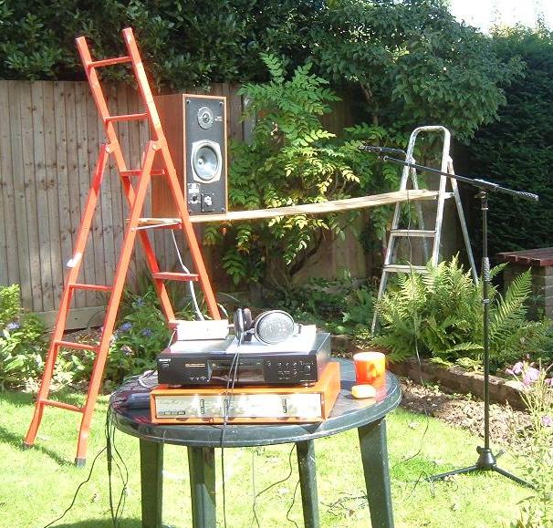
The in-room measurements discussed above provided some evidence of the suspected sensitivity mismatch between the tweeter and woofer. However it was not possible to do more than guess at its magnitude on account of the large fluctuations in the measured frequency response. Consequently more accurate estimates were necessary, and these were facilitated by performing measurements in near-free field (anechoic) conditions rather than in a room. One does not need an anechoic chamber to get useful results. Instead, one simply does the measurements outdoors. A picture of my measurement setup in a corner of the garden is shown in Figure 8.
Figure 8. Near-free field measurement setup outdoors
Desirably one should site the speaker and microphone as far away from boundaries as possible, and the situation depicted was somewhat better than it might appear because the visual perspective of this shot has turned out rather perversely on account of the zoom lens. The fence was further away than it seems, and the measurement axis between speaker and microphone was deliberately angled off the perpendicular to the fence to avoid the largest reflections from it reaching the microphone.
The frequency response measured in this near-free field situation is at Figure 9. Additional bass rolloff below about 150 Hz was imposed this time by inserting a high pass filter between the microphone output and its preamplifier. This reduced wind noise which might otherwise have saturated the electronics, because most capacitor microphones have a response down to very low frequencies of a few Hertz.
Figure 9. Loudspeaker frequency response measured in near-free field conditions out of doors
You can see immediately that none of the gross room-type reflections observed earlier in Figure 5 have reappeared this time. Indeed, the plot is almost as clean as that of the averaged white noise source signal itself (see Figure 3) and the measured response of the Sennheiser headphones (Figure 4). This confirms that the measurements were undeniably performed in near-free field conditions. Although the frequency response is not flat, it is now possible to see and measure the difference between the woofer response and that of the tweeter more readily. The woofer response occupies the first 3 kHz of the plot, with the remainder representing the tweeter. It was therefore confirmed that the difference between them was indeed at least 6 dB, though probably somewhat greater.
You might also like to play the "Spot the Crossover Frequency" game again. Do you find it surprising that, even with this much cleaner spectrum, it is still impossible to detect it by eye? It cannot even be seen in a higher resolution plot in which the expanded frequency scale only goes up to 4 kHz (Figure 10). The same applies to baffle effects in that there is no visible evidence of the spectrum periodicities which theory predicts. So in both cases perhaps we ought not to put so much emphasis on either of these matters if they are not obvious even in near-free field measurements.
Figure 10. Loudspeaker frequency response measured in near-free field conditions - LF region below 4 kHz
Some further experiments were done including subjective listening tests involving comparison with the Sennheiser headphones, and it was concluded that a tweeter attenuation relative to the woofer of 8 dB was undeniably preferable to the 6 dB initially suggested by the in-room frequency response of Figure 5. This is compatible with the cleaner near-free field result shown in Figure 9 which suggested a somewhat greater discrepancy in sensitivities. 8 dB is a considerable amount (a power reduction by a factor of 6.3), so no wonder the speakers sounded too 'bright'. But because of the criticality of equalising the sensitivities of the woofer and tweeter, I decided to incorporate a switchable attenuator between the high pass crossover and the tweeter which reduced the tweeter drive by zero, -3 and -8 dB. Having more than one fixed value of attenuation is advantageous in a real room setting.
It is also worth mentioning that the entire process described above was repeated with the other loudspeaker cabinet. Even high quality drive units such as the KEF ones used here are subject to manufacturing tolerances, and it was found that the other tweeter was about 3 dB more sensitive than the one discussed above. Consequently it needed an even higher attenuation to achieve equalisation with the woofer. This explains why the drivers used in the highest quality loudspeakers should have been matched by selecting them from a production batch, and if they were not you are well advised not to part with your money.
Contrary to what is often assumed, one cannot simply insert a series resistor between the output of the crossover network and the tweeter to reduce the drive to the latter. This is because the component values in the crossover are usually calculated assuming a resistive load equal to the nominal tweeter impedance. In this case a series resistor would have introduced a hump in the treble response of about 4 dB just above the crossover frequency, and the 'knee' and rolloff slope of the high pass filter characteristic would also have been degraded (I checked these predictions experimentally). A series resistor reduces the damping of the inductor in the high pass crossover network by the tweeter impedance, allowing the inductor to resonate with an excessive Q-factor and thus generate the unwanted hump and other undesirable effects.
Instead, it is necessary to use a resistive matched network which presents the required design resistance to the crossover while introducing the desired attenuation. Such a network is sometimes called an L-pad. Because two values of attenuation were required, two L-pads were necessary. A necessary remark is that the switch by which they were selected had to be chosen to have an adequate current rating. The T27 tweeter can handle 8W of continuous power, and as its nominal impedance is 8 ohms this means the maximum continuous current it can accept is about 1A rms. Most rotary wafer switches are not rated at anything approaching this figure and it is difficult find a component which is suitable. However RS Components currently offer one by Lorlin rated at 2A (stock number 665-843). Design details for L-pads are given in Appendix 1 because much information on the Internet is incorrect.
The circuit diagram of the complete 3-position switched attenuator incorporating two L-pads is shown in Figure 11. L-pad A gives 3 dB of attenuation and L-pad B gives 8 dB in round figures. The resistor values are written using European notation which does not seem to be understood in some other countries, so to be clear, 1R8 means 1.8 ohms, 27R means 27 ohms, etc. The resistor values for the other loudspeaker were different because of the different sensitivity of its tweeter as mentioned above. All resistors were rated at a minimum power dissipation of 3W. It is worth noting that the additional resistance between the crossover and the tweeter endowed by an L-pad is beneficial to crossover performance. The tweeter voice coil inductance and its resonant frequency combined with the crossover network impedances can result in undesirable artefacts which can be mitigated by the isolating effect of the additional resistance in the L-pad. It means that the crossover now works into a better approximation to a purely resistive load, which is frequently though incorrectly assumed when designing it. As already mentioned, I do not get too exercised about the design of crossovers because other issues such as room effects are so detrimental to overall performance as we have seen. However there is no harm in pointing out this incidental advantage intrinsic to the use of L-pads besides their primary function of realising a matched attenuator.
Figure 11. Switchable tweeter attenuator using two L-pads, giving three sensitivity settings in all
The switched tweeter attenuator with its aluminium control knob can be seen in the picture of the completed loudspeaker (Figure 12). This also shows the KEF 'acoustic contour control' for the woofer. Together these two controls provide a useful and unusual degree of flexibility when optimising the performance of the loudspeakers against different programme material in a room.
Figure 12. The completed loudspeaker with switchable tweeter sensitivity (aluminium control knob)
Some people have asked whether a rotary L-pad of the type widely available commercially could be used instead of the switched system described above. The answer is "probably", but only provided it is constructed very robustly . The main problem with the potentiometers in some of these items is that the resistance between the wipers and the resistance elements increases over time, either because corrosion sets in or because tarnish builds up on a silver-plated wiper. The contact resistance at this point must remain effectively zero, and this is asking a lot of a mechanical wiping contact which must carry substantial currents measured in ampères. But it will still be necessary to calibrate the L-pad so that you know what attenuation you are getting at any position of the control knob, and you also need to know what attenuation you need in the first place. Therefore a measurement process similar to that described above will still be necessary if you are to achieve something better than merely adjusting the system by ear alone.
Note that an L-pad cannot be used to reduce the drive to a woofer. Therefore if you have a woofer which is more sensitive than the tweeter, which is the reverse of the problem discussed in this article, you cannot equalise the two using any form of passive attenuator. This is because a woofer must be driven from a source impedance not greater than a very small fraction of an ohm, which means it must always be connected direct to the amplifier (through a very low impedance crossover) using leads of negligible resistance. Otherwise the motion of the cone will be insufficiently damped and you will experience an unpleasant boomy, peaky and poorly defined bass response which will be especially noticeable on the lower notes of a digital organ. The problem in this case can only be solved by using bi-amping in which the woofer and the tweeter are driven from separate power amplifiers with the necessary equalisation being applied at their inputs. However this approach does have the advantage that it removes the need for a crossover network should you dislike them.
If you have read this far you will probably have formed the view, correctly, that I regard subjective assessments of audio equipment as virtually worthless. Therefore I will try not to fall into the same trap myself, other than to say that the modified loudspeakers now sound adequate if not respectable. They are certainly much better than they were and they no longer tire the ear because the former excessive high frequency 'brightness' has gone. Nevertheless the measurements described in this article not only pointed the way towards improving their performance but they also showed up their remaining limitations. For instance, the measurements in near-free field conditions (Figure 9) demonstrate that the frequency response is not exactly flat, but neither was that of the expensive Sennheiser headphones (Figure 4), at least when measured with the particular microphone used here. However reducing the tweeter response in the manner described improved matters of course. It is difficult to compare the results here with those for other loudspeakers because such results are seldom made available, either because the measurements were not made to start with or because manufacturers are unwilling or embarrassed to disclose them.
A thesis of this article is that room effects are so dominant that it is pointless getting too hung up about some details of loudspeaker design and performance, such as the minutiae of crossovers and baffle effects. But one rarely comes across actual measurements such as those presented here to illustrate this point. The consequence is that only major shortcomings can be detected by the ear in a real room, such as that which initiated this work in the first place to do with the mismatched sensitivities of woofers and tweeters. (Another shortcoming which is independent of the room is loudspeaker distortion, because both harmonic and intermodulation distortion result in additional radiated frequencies not present in the source signal. If distortion is excessive the ear can detect the distortion products regardless of room effects because the latter cannot transfer source power into spurious frequencies, no matter how extreme the effects might be. However distortion was not an issue with these loudspeakers).
These loudspeakers were mainly intended for duty with digital organs, and in this application their extreme bass response and power handling capacity were inadequate. This will be true for any comparable system using ordinary hi-fi drivers and enclosures, and one therefore has to use separate sub-woofers to handle the lowest frequencies. A detailed discussion of the problems of radiating the extreme bass from electronic organs appears elsewhere on this website [1]. Apart from this limitation the speakers have proved very acceptable for use in the medium and high frequency regions above about 40 Hz, and at least as good as any similar commercial system which I have come across in any price bracket. By "similar" I mean a sealed box system of similar physical size using two drive units. Moreover, the range of adjustment described here is rarely found. The speakers also perform well in general hi-fi applications.
The main conclusion is that you can only determine what is wrong with an unsatisfactory loudspeaker by performing measurements on it. But as this article has shown, this is a time consuming, difficult and more or less expensive business in the course of which you literally have to get your hands dirty. So perhaps it is not surprising that so few people bother to go that way.
Notes and References
1. "The Electronic Reproduction of Very Low Frequencies", an article on this website, C E Pykett, May 2004
2. The dimensions corresponding to the sketch in Figure 6 were:
3. "Wet or Dry Sampling for Digital Organs?", an article on this website, C E Pykett, April 2010
4. On average, the amplitude excursion of each frequency component in white noise is symmetrical about the mean value over time, and it is confined to the range M/30 to M(1 + 29/30) approximately, where M is the mean. This range when expressed in decibels becomes -30 to +6 dB in round figures relative to the mean, which is what is seen in the actual white noise spectrum in Figure 2. Note how the symmetrical excursions when measured on a linear amplitude scale become highly non-linear when converted to decibels. Therefore when computing the mean value the linear amplitudes must be used, not the logarithmic ones, otherwise the apparent mean value itself would change.
5. The periodic interference ripples in the in-room spectra (Figures 5 and 7 above) due to standing waves are actually sinusoidal. However they take on a different shape when plotted on a logarithmic scale, as was done here where the vertical axis represents decibels. This effect is shown in the diagram below where a sine wave is plotted using linear values (blue curve) and logarithmic ones (pink curve). It can be seen that the pink curve approximates well to the shape of the standing wave ripples in Figures 5 and 7.
A sine wave plotted using a linear scale (blue curve) and a logarithmic one (pink curve)
Appendix 1 - L-pad attenuator design
Design information concerning L-pads on the Internet is frequently wrong. Be especially wary of the 'calculators' included in web pages as these do not always give the correct results. Examining the embedded code shows that a common mistake occurs when converting the desired attenuation expressed in dB into the factor required by the design equations - designers frequently get confused between power and voltage, for which the conversion results are grossly different. The design equations are simple but one needs to keep a clear head especially where decibels are concerned.
Figure A1. Switchable tweeter attenuator using two L-pads, giving three sensitivity settings in all
Figure A1 is a repetition of the diagram presented earlier in the main text showing the component values of the two L-pads. The resistor values to achieve a given attenuation A (defined as below) for a tweeter of nominal impedance Z are given by:
R1 = Z(1 - A) (1) R2 = ZA/(1 - A) (2)
R1 and R2 are in ohms if Z is in ohms.
To pre-empt possible controversy as to whether these equations are correct, you can do a simple experiment with a battery and test meter described at the end of this Appendix to prove that they are.
A is the desired attenuation, defined here as the ratio of the output voltage across R2 when shunted with the tweeter divided by the input voltage applied to R1. Thus A is always less than 1. It could be argued (correctly) that this is a definition of gain rather than attenuation, but because many people object to a 'gain' of less than unity, I have called it attenuation here. I have found from experience that this is a parameter whose definition can never satisfy everyone, so apologies if you find it confusing.
If the attenuation is expressed in decibels the conversion equation is:
A = 10 B/20 = 10 ^ (B/20) = "ten to the power of B/20" (3)
where B is the desired attenuation expressed in dB. This is the attenuation to be applied to the voltage (not the power) appearing at the crossover output before it reaches the tweeter. B must be a negative number, so if you want an attenuation of 6 dB, say, then you must put a minus sign in front of it when calculating the equation above. Otherwise the value of A you get will be wrong because it will be greater than 1 and the equations (1) and (2) for R1 and R2 will then be nonsense. The correct value of A is 0.5 (using equation (3)) in this example where B = -6 dB, thus A is less than 1 as required. (If you had not made B negative, A would be 2 and the resistor values would then turn out negative).
From all this, maybe now you can appreciate why much of the design information for L-pads on the Internet is wrong!
You can check your calculations by doing them in reverse i.e. using the resistor values to get back to the corresponding attenuation. This should be the same figure you started with of course. The 'reverse' equation is:
A = ZR2/(R1R2 + ZR1 + ZR2) (4)
The value of A which you get should be less than 1. Putting it into the following equation will then give the corresponding value in dB, which should be negative:
B = 20log10 A (5)
where log10 means "logarithm to the base 10".
To get familiar with these equations you might like to try using the resistor values for 'L-pad B' in the diagram above to work out its attenuation figure:
From the diagram, R1 = 4.7Ω, R2 = 5.1Ω and Z = 8Ω (tweeter impedance). Using equation (4), A = 0.4 (less than 1 as required), and using equation (5) B = -8 dB (negative as required). These have been rounded to approximate ('near enough') values.
Putting this value of A back into the equations for R1 and R2 (equations (1) and (2)) gives R1 = 4.8Ω and R2 = 5.3Ω, which are near enough to the values we started with. So everything checks out OK.
Experimental check of the design equations In view of the appearance of incorrect design details elsewhere, it is easy to verify experimentally those given here in equations (1) and (2). Simply make up a network of three resistors and do some quick measurements on it with a battery and a multimeter.
For example, let the design impedance (Z) of the experimental L-pad be 10 kΩ. Normally this would be the tweeter impedance of a few ohms but we cannot easily use such low values here for practical reasons. Let the desired attenuation (A) be 0.4. Then R1 = 6kΩ using equation (1) - use the nearest preferred value of 6.2kΩ. And R2 = 6.67kΩ using equation (2) - use 6.8kΩ. Connect a third resistor of 10kΩ in parallel with R2 to act as the design load.
Using a resistance meter measure the input resistance of the network between the input to R1 and the bottom end of R2. It will be close to 10kΩ as required. The result will be exact if you used exact values for R1 and R2.
Remove the meter and connect a battery to the same terminals instead. Measure the voltage at this point - say V. Then if you measure the voltage at the output - across the 10kΩ resistor - it will be close to 0.4V as required.
So if anyone insists their equations are correct but they are different to mine, just do this simple experiment to decide who is right!
|