


|
|
|
The Effect of Organ Pipe Scales on their Harmonic Spectra
"Perhaps scaling is better judged as a measure of intent than of actual results" Stephen Bicknell [3]
Posted: 14 February 2016 Revised:
15 March 2016
Abstract. This article shows how the effects of organ pipe scaling laws can be related objectively rather than subjectively to changes in their tone quality across a rank. This fills a gap in organ building practice and in the literature, where little exists which quantifies the choice of pipe scale on the tonal effects of an organ stop. The tone quality of a pipe is reflected in its frequency spectrum, but there are three major difficulties in using the spectrum directly. Firstly the amplitudes of the harmonics exhibit gross scatter which varies unpredictably from pipe to pipe. Secondly the harmonic pattern of an individual pipe is not invariant but depends on listening position within the building, because the perturbing effects of standing waves on each harmonic are unique to a particular location. Thirdly a spectrum contains many harmonics, therefore attempting to define it using their amplitudes is unmanageable.
These problems were solved by approximating to the pattern of harmonic amplitudes using linear trendlines. Only two lines are required to represent most, if not all, organ pipe spectra. Thus only three parameters are required to define a spectrum, namely the point of intersection of the two lines and their slopes. Trendlines are less strongly affected by the factors which perturb the individual harmonic amplitudes because the factors are more or less random, therefore the lines tend to 'iron them out'. Consequently the three trendline parameters form a robust data triplet for approximating to the pattern of harmonics in a spectrum.
It is shown how the trendline parameters vary across the key compass for a diapason organ stop whose pipe diameters followed a Töpfer-type progression in which they halved at every sixteenth pipe. The parameters were estimated from spectra derived from recordings of the pipes in situ in a building, and variations of the three parameters across the keyboard were compatible with those expected from this scaling law. For instance, the level of the second harmonic increased systematically towards the bass and decreased towards the treble. This behaviour reflected the variation in pipe diameter whereby the bass pipes were narrower (relative to their speaking length) compared with those higher in the compass. Thus it was possible to observe the operation of the scaling progression quantitatively in terms of its effects on tone quality across the compass, perhaps for the first time.
Contents (click on the headings below to access the desired section)
The relative importance of pipe scale and voicing adjustments
Much attention has been paid to organ pipe scales for hundreds of years. This is understandable because the scaling applied to a rank of organ pipes profoundly affects how it sounds in the building, and if the scales of the various stops are not optimum a voicer can only compensate for the resulting tonal defects to a limited extent since pipe dimensions obviously constrain mouth dimensions. They also define some aspects of organ pipe physics such as the retinue of natural resonances of the air column, and these have a critical influence on tone quality. The scale of an organ pipe is a measure of its cross-sectional area to its speaking length but the two parameters do not, indeed they cannot, vary across a rank in the same way. Taking an example, while pipe length halves every octave or every twelfth pipe, the diameter of a cylindrical pipe varies more slowly. Typically the diameter of a diapason (principal) pipe might halve at every sixteenth note, that is at the interval of a major tenth rather than at the octave. Scaling laws such as this (and there are many others) are necessary to encourage the acoustic power and tone quality of the pipes to remain subjectively of a piece across the rank as far as possible. If the diameters vary too rapidly the pipes lose power towards the treble, and they also become scratchy and shrieky in tone because they get too narrow. Conversely, they sound ponderous, dull and lifeless if the diameters vary too slowly. The physics behind this behaviour is explained at a simple level in another article on this site [1].
The venerable backdrop of organ building history which informs today's pipe scaling practices can be traced back earlier than the seventeenth century. For much of this time span the understanding was empirical and based on a body of experience built up largely by trial and error. Not only was there little appreciation of organ pipe physics but an essential ingredient to the mix, logarithmic arithmetic, did not arrive until later. However master organ builders such as Arp Schnitger in the late 1600s and Gottfiried Silbermann some fifty years later did not allow this to cramp their style unduly, and their work shows clearly how they were addressing the problem generally successfully to the extent that Ralph Downes was at pains to apply their insights to the Royal Festival Hall organ in London in the 1950s.
So there is no doubting the profound effect that pipe scales have on the sound of an organ but, perhaps surprisingly, that is about all that can be said. In spite of the colossal amount of work devoted to the subject at both practical and theoretical levels over hundreds of years, next to nothing exists which quantifies objectively the consequences of the choice of pipe scale on the effect of a particular organ stop. Occasionally one comes across attempts to measure the amplitudes of the first few harmonics of each pipe in a rank, but this is far removed from quantifying their timbre and it does little more than illustrate the standing wave patterns in the building. There is therefore a missing link in the chain. Even today one cannot go beyond vague subjective assertions such as "this choice of scale confers an attractive bloom to the mid-range". Such statements convey little useful information, thus they only provoke largely sterile debate. In an attempt to go beyond this, sometimes organ builders employ acousticians to characterise the frequency response of a building in terms of its peaks and troughs in the hope that they will be able to devise pipe scales which compensate for the variations. Yet little or nothing is done subsequently to quantify whether the resulting instrument actually satisfies the design brief. The main reason for this is that a broadly accepted methodology, indeed any methodology, for doing it does not exist. This vindicates Stephen Bicknell's remark quoted at the head of this page. Consequently it is this shortcoming which the article attempts to address by relating pipe scale to tone quality across a rank in a particular building in an objective manner, and the techniques and results described here are believed to be original.
Because an organ pipe can emit sound indefinitely, it is well known that the harmonic structure of its steady-state acoustic emission dominates its tone quality or timbre as perceived subjectively. Other factors such as attack transients also play a part, but these are not immediately related to pipe scale in the intimate way that scale affects the frequency spectrum of a pipe. The distribution of the acoustic power radiated by a pipe among its harmonics also influences its perceived loudness, which is a subjective measure not solely determined by its broadband sound pressure level. Therefore the frequency spectrum is a most important parameter when pursuing a causal link between pipe dimensions (i.e. scale) and their effects on tone quality and loudness. Unfortunately, however, a spectrum is not characterised by a single parameter to which a specific value can be assigned. On the contrary, it is not unusual for a spectrum to contain over 30 harmonics, each of which has a frequency and an amplitude, which means that upwards of 60 numbers are required to specify such a spectrum numerically. It verges on the impossible to relate such a complex entity to pipe scale without reducing the data burden in some way. Moreover, the amplitude of each harmonic is not solely a property of the pipe but also of the room or auditorium into which it speaks. This is because reflections from the surfaces in the room generate standing waves which either reduce or augment the level of each harmonic in a unique way at a particular listening position, a phenomenon which results in continuous changes in the tone quality of a pipe if one moves around the room. Therefore, as is well known, each member of the audience at an organ recital will receive a different impression of how the instrument sounds. The effect is illustrated in the sound clip below of a Trompette reed pipe as the recording microphone was moved around in the building:
If you have the inclination and facilities, you can replay this recording into a real time spectrum analysis app on your computer and observe how the levels of the various harmonics rise and fall as the microphone position varies. In fact it is the building which imposes much of the 'scatter' observed in organ pipe spectra. Spectra obtained from pipes sounding in anechoic conditions have spectral envelopes which are usually much smoother, rendering them less 'ragged' in appearance. Nevertheless, we have to listen to organs in buildings rather than in anechoic chambers and therefore pipe scales have to be chosen to suit the building despite the more or less random scatter which the building imposes on the harmonic amplitudes of each pipe, and differently at each listening position.
So the problem is this. How can we relate pipe scale to the emitted frequency spectrum of a pipe and thus draw conclusions as to how scale affects tone quality and loudness, bearing in mind that a spectrum apparently requires a lot of numbers if we are to capture it quantitatively? A more immediate difficulty is that the question itself might seem nonsensical because we have just seen (and heard from the recording above) that there is no unique and unambiguous spectrum of a pipe when auditioned in the real environment of a building. Yet there is hope for a successful outcome because the ear and brain somehow seem to transcend these difficulties. For instance, there is usually little doubt when an unsatisfactory organ is badly scaled. We can also assign without difficulty the single label 'trompette' to the continuously-varying sound of the pipe in the recording above, despite the fact that its instantaneous harmonic structure varies dramatically with listening position - our remarkable auditory apparatus is not particularly confused by the changes in timbre which occur even though, paradoxically, we can readily perceive them as they happen.
Thus there are actually two requirements. The first is to capture the essentials of the harmonic structure of a an organ pipe, its frequency spectrum, using just a few numbers rather than the plethora of data which the spectrum itself contains in the amplitudes and frequencies of all its constituent harmonics. These numbers must not be unduly influenced by the spectral scatter which occurs among the harmonic amplitudes of an organ pipe in practice, nor by the changes which occur with listening position. The second requirement is then to relate these few numbers to the scale of the pipe which produced the spectrum in the first place. These are not trivial prerequisites, and they will be now be considered in turn.
A case study was chosen to illustrate the points made in this article. It was a 'large' open diapason stop in an organ built in the early twentieth century. This was selected deliberately because it employed the scaling precepts introduced into England by Edmund Schulze, who in turn was a disciple of the practices advocated by J G Töpfer. It was he who suggested in his well-known book [2] the use of the scale mentioned above in which the pipe diameters of a diapason rank should halve at every sixteenth note, and he gave full details in the public domain for the first time of how to implement it. Although uniform scales such as those of Töpfer have since attracted criticism on the grounds that they can too easily lead to the nineteenth century 'factory organ' with its bland and undifferentiated sound, they still underpin the baseline (Normal Scaling or Normalmensur) against which other scales used today are referenced. In any case, Töpfer's scaling rules themselves are still widely employed by pipe makers and organ builders today. Thus in this diapason stop we have an extant Edwardian example of Töpfer's sixteenth-note scaling progression as applied in practice.
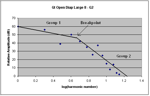
Figure 1. Spectrum of a Large Open Diapason pipe (tenor G). Two trendlines are also shown.
The blue dots in Figure 1 show the harmonic amplitude spectrum of the tenor G pipe (the G below middle C) from this diapason rank. The scatter among the points is typical of that observed with organ pipe spectra, and it is largely due to the effect of the building as described earlier. If the recording microphone had been moved a completely different pattern would have been captured, yet the ear would still have been able to decide that the sound was that of an open diapason. It is this remarkable fact that first requires investigation. Observe that the pattern of harmonics falls naturally into two regions labelled Group 1 and Group 2 which have been approximated by the two trendlines drawn on the graph. It is remarkable that this two-group structure is common to all of the spectra I have examined over some forty years of research, embracing flute, diapason, string and reed pipes. The two lines intersect at a point which is called the 'breakpoint' here.
The justification for using a trendline approximation to represent a spectrum is that no two pipes of any organ stop sound exactly the same in terms of their timbres, even adjacent ones, and moreover the sound of any one pipe varies significantly at different points in the building as the previous discussion showed. Therefore there is no such thing as 'the sound' of an organ pipe in practice in the sense of it being unique or invariant. It is this intrinsic variability which enables trendlines to capture the essentials of spectra which are subject to these perturbations, because the lines themselves are not influenced as strongly as are the individual harmonics by random variations. They tend to ' iron out' the scatter among the harmonics. An important feature of trendlines is that they enable a spectrum to be represented using only three numbers in this case - these are the breakpoint or harmonic number at which the two lines intersect and the slopes of each line measured in decibels per octave. Thus the spectrum in Figure 1 was characterised by a number triplet with the values 4.5 for the breakpoint expressed in terms of harmonic number, -6 dB/8ve for the slope of the Group 1 trendline and -23 dB/8ve for the Group 2 slope. This is very much less than the 28 numbers which would otherwise have been required (the amplitudes and frequencies of 14 harmonics) and therefore it is much easier to handle. So we have answered the first question posed in the previous section - how to capture the essentials of the harmonic structure of a an organ pipe using just a few numbers. An expanded discussion of trendlines applied to organ pipe spectra appears in another article on this site [4].
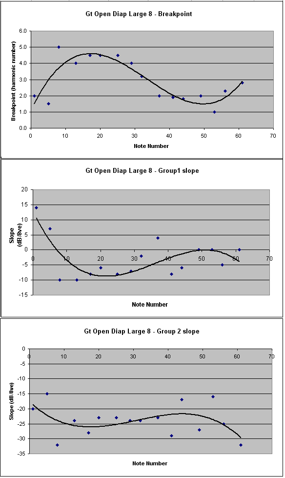
The second question above required the spectrum, now represented economically in trendline form, to be related to pipe scale. This was done as follows. The spectra of sixteen pipes equally spaced across this diapason rank (three per octave) were computed and trendlines derived for each one. In each case the three numerical values defining the two lines were measured and then plotted in terms of their position in the key compass. This resulted in the three graphs shown in Figure 2, one for each trendline parameter. The horizontal axis of each graph represents note number running from 1 (bottom C) to 61 (top C).
Figure 2. Large Open Diapason - variation of trendline parameters across the key compass
The 16 individual values of each trendline parameter (the breakpoint and the two line slopes) are represented by the blue dots in the respective graph. As with the individual spectra themselves there is quite a lot of scatter in evidence. However fitting curves to the graphs (the black lines) enabled some interesting behaviour to be identified. Firstly consider the slopes of the Group 2 trendlines as plotted in the bottom graph. These lines are those associated with the high order/low amplitude harmonics in each spectrum as shown earlier in Figure 1, and they do not vary greatly across much of the compass despite the outlying points at each end. The mean value is about -24 dB/8ve which accords with what the eye can detect across the central region of the compass. It is possible that the decrease in trendline slope towards the bass and the increase towards the treble, suggested by the black curve, are simply artefacts due to the random scatter in the data in these regions rather than indicating systematic behaviour. However such behaviour is nevertheless sensible because it suggests that more harmonics will be emitted by the bass pipes because the line slope becomes less steep than in the treble, where the reverse will apply. This accords with what one would expect from everyday experience, but more to the point this is precisely the behaviour encouraged by a scaling law such as that of Töpfer which makes the bass pipes narrower relative to their speaking length compared with pipes in middle of the compass. Narrower pipes emit more harmonics, other factors being equal. Towards the treble the scaling law makes the pipes wider, thus they emit fewer harmonics, a feature also suggested by the graph. It is therefore probable that this graph is indeed reflecting spectral, and thus tonal, characteristics across the key compass which are related to the Töpfer scaling applied to this pipe rank.
The other two parameters, the breakpoint and the slope of the Group 1 trendline, show an interesting feature towards the bass end of the compass. The breakpoint value decreases markedly, whereas simultaneously the Group 1 slope changes rapidly from a negative value to a positive one. Taken together, these result in significant changes in the spectra towards the bass. Higher in the compass a typical spectrum was shown in Figure 1, whereas in the bottom octave it becomes quite different. To illustrate this, the spectrum for the bottom note is shown in Figure 3 below.
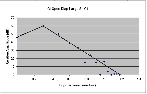
Figure 3. Spectrum of a Large Open Diapason pipe (bottom C). Two trendlines are also shown.
Note how the Group 1 trendline now has a positive (upwards) slope whereas formerly it was negative. The breakpoint has also reduced from its former value to lie at the second harmonic. These changes result in the pipe emitting a second harmonic of considerably higher relative amplitude than those further up the keyboard, and this effect also applies to some of the subsequent harmonics. For this pipe the second harmonic has reached five times the amplitude of the fundamental (14 dB), and even the third harmonic is about 1.6 times stronger (4 dB). This is quite different to pipes higher up the compass whose spectra are typified by that shown in Figure 1, where the strongest harmonic is the fundamental itself. This behaviour results in the bass pipes of this diapason stop sounding much brighter and less ponderous than they would otherwise have done had no scaling been applied. This is partly a consequence of the relative narrowing of the pipes towards the bass conferred by a Töpfer-type scale. Therefore, again the data here are reflecting clearly certain tonal characteristics which are related to the scaling of this rank.
To summarise, the curves in Figure 2 show how the spectra and thus the tone quality of this diapason stop vary across the key compass. This was only made possible through the use of three trendline parameters to represent the essentials of each spectrum, because it would otherwise have been impractical to reach any conclusions at all. It was further shown that some aspects of the curves are clearly compatible with the scaling law applied to the pipe rank. We have therefore been able to show how the frequency spectra, and thus the tone quality, varied across the compass. We have also suggested how the variations might relate to the scaling of this diapason stop. These conclusions and the means of deriving them are believed to be original.
The relative importance of pipe scale and voicing adjustments
The power and tone quality of an organ pipe are influenced not only by its scale but also by adjustments made by the voicer. For instance, the amplitudes of the early harmonics relative to the fundamental are modified by cut-up (mouth height as a proportion of its width), the sharpness of the upper lip, wind pressure at the languid (adjusted by varying the size of the foot hole) and varying the angle at which the air jet hits the upper lip (adjusted by raising or lowering the languid). Therefore it can be argued that the voicer can compensate for an unsatisfactory scaling law, and to some extent this is true. It is also true that voicing adjustments will modify or perhaps obscure effects due to scaling as far as an individual pipe is concerned.. However the effect of scaling nevertheless remains important for at least two reasons. The first is because of its cumulative effect across a rank of pipes. With a uniform scale such as that of Töpfer the pipes halve in diameter several times across the compass, thus a small change in the law (such as halving on the seventeenth rather than the sixteenth pipe) will have major consequences for the diameters of pipes higher in the compass. This will be reflected in their harmonic spectra and thus in their tone colour. The same is true of the power of the pipes, which is strongly related to mouth size, and this in turn is constrained by pipe circumference and thus scale. Voicing adjustments cannot compensate completely for such major changes across an entire rank of pipes resulting from scales which might differ only slightly in terms of their diameter-halving interval.
The second reason why scale is so important is that there are several aspects of organ pipe physics which depend critically on pipe dimensions, and these cannot be modified by the voicer because they are fixed once a pipe has been made. The most important aspect is the retinue of natural resonant frequencies of the pipe. These are anharmonic and they strongly influence tone quality because of the way they interact with the harmonics generated by the air jet at the mouth. They are determined almost entirely by the length and cross-sectional area of the pipe, in other words by its scale. A detailed discussion of these matters is available in another article on this site [5].
Thus, although the voicer can indeed adjust the speaking behaviour of a pipe, he can only do so within relatively narrow limits. What we hear from any pipe is a combination of its scale and how it has been treated by the voicer, but the influence of scale is profound and it goes beyond what the voicer can do. Once a pipe has been made, much of its tone quality has already been determined once and for all. The curves in Figure 2 obviously represent a combination of these two effects, scaling and voicing, rather than pipe scale alone. But because scale becomes such a dominant factor when a rank is considered as a whole, as here, I suggest that its effects are indeed reflected in these data in ways which have been brought out in the previous discussion.
This article has shown how the effects of organ pipe scaling laws can be related objectively rather than subjectively to changes in their tone quality or timbre across a rank. This fills a gap in organ building practice and in the literature, where little exists which quantifies the choice of pipe scale on the tonal effects of a particular organ stop. The tone quality of an organ pipe is reflected in its frequency spectrum, but there are three major difficulties in using the spectrum directly. Firstly the amplitudes of the harmonics exhibit gross scatter in any one spectrum, and this varies unpredictably from pipe to pipe. Secondly the scattered harmonic pattern of an individual pipe is not invariant but depends on listening position within the building, because the perturbing effects of standing waves on each harmonic are unique to a particular location. Thirdly a spectrum contains many harmonics, therefore attempting to define it using their amplitudes is unmanageable.
These problems were solved by approximating to the pattern of harmonic amplitudes using linear trendlines. It has been found that only two lines are required to represent most, if not all, organ pipe spectra. This means that only three parameters were required to define a spectrum, namely the point of intersection of the two lines and their slopes. Trendlines are less strongly affected by the factors which perturb the individual harmonic amplitudes because the factors are more or less random, therefore the lines tend to 'iron them out'. Consequently the three trendline parameters form a useful and robust data triplet for approximating to the pattern of harmonics in a spectrum.
It was shown how the trendline parameters varied across the key compass for a diapason organ stop where the pipe diameters followed a Töpfer-type progression in which they halved at every sixteenth pipe. The parameters were estimated from spectra derived from recordings of the pipes in situ in a building. Variations of the three parameters across the keyboard were compatible with those expected from this scaling law. For instance, the level of the second harmonic increased systematically towards the bass and decreased towards the treble. This behaviour reflected the variation in pipe diameter whereby the bass pipes were narrower (relative to their speaking length) compared with those higher in the compass. Thus it was possible to observe the operation of the Töpfer scaling progression quantitatively in terms of its effects on tone quality across the rank, perhaps for the first time. In simple terms it prevented the bass pipes becoming woolly and ponderous and the treble ones from sounding scratchy and shrieky, but this article has shown how to justify this statement with numbers
In explaining the results solely in terms of pipe scale, no account was taken of the voicing adjustments which would undoubtedly have affected the timbre of some pipes. However it was pointed out that the influence of scaling is profound and it goes beyond what the voicer can do when a complete rank of pipes is considered, as here. Once a pipe has been made, much of its tone quality has already been determined once and for all. In particular, its retinue of natural frequencies is largely determined by its length and cross-sectional area, in other words by its scale, and these dimensions lie beyond the control of a voicer. The natural frequencies strongly influence tone quality because of the way they interact with the harmonics generated by the air jet at the pipe mouth.
It is believed this methodology and results have not been reported previously, and that therefore they are original.
1. "How the Flue Pipe Speaks", an article on this website, C E Pykett 2001.
2. "Die Orgelbaukunst" (The Art of Organ Building), J G Töpfer, Weimar 1833.
3. "Scaly Monsters", Stephen Bicknell, number 4 of 6 articles published in Choir & Organ in 1998-9 under the heading 'Spit and Polish'.
4. "Some novel observations on organ pipe sounds and their frequency spectra", an article on this website, C E Pykett 2015.
5. "The End Corrections, Natural Frequencies, Tone Colour and Physical Modelling of Organ Flue Pipes", an article on this website, C E Pykett 2013.
|