Double ambience - the Achilles Heel of sampled sound synthesis  

Colin Pykett

Posted: 24 March 2017

Revised: 25 March 2017

Copyright © C E Pykett 2017

Abstract.  Sampled sound synthesis is used widely in digital organs and universally in virtual pipe organs. Usually the samples are recordings of actual organ pipes, and therefore manufacturers frequently claim that their products sound indistinguishable from the real thing. However this article shows that this claim is questionable for at least one reason - double ambience. This term reflects the fact that the recordings are made in one room whereas the instruments are played in another. It is well known that room ambience imposes often gross distortions on the harmonic amplitudes which constitute the frequency spectrum of an organ pipe, and the distortion varies dramatically over distances of a few centimetres. Therefore when the ambiences of two rooms effectively in series are involved, the already-distorted waveforms in the memory of a digital organ will be distorted in a different way for a second time when the instrument is played. Aural examples of the effects of single and double ambience on reed and diapason tones are presented to illustrate the problem. Double ambience is in fact a wholly artificial listening environment which never arose in human experience until the advent of broadcast audio and recorded sound. Consequently it would unsurprising if our brains have not evolved with the ability to fully process sounds which come to us via two stages of ambience. If so, then maybe this is one reason why some people find sampled-sound digital synthesis inherently unsatisfactory and why they can readily identify digital organs as those which do not use pipes.

Contents
(click on the headings below to access the desired sections)

Introduction

The ambience of a single room - a demonstration

The Amplitude Transfer Function (ATF) of a room

Double room ambience - a demonstration

Concluding remarks

Appendix 1 - The technical quality of Boner's results

References

Introduction

At the time of writing (2017) sampled sound synthesis is by far the most common means of simulating the pipe organ. Most current digital organs and all current virtual pipe organs use it, and manufacturers make much of the fact that the sounds of real pipes recorded from actual instruments can be called up instantaneously as a performer presses the keys. They are therefore not slow to claim that the resulting sounds are indistinguishable from the real thing.

Is this true, or are certain factors overlooked which work against it? There is no doubt that the hype disguises at least one awkward fact which I have never seen mentioned. Obvious when you think about it, this concerns room ambience, the aural effects which a room or an auditorium imposes on sounds arising within it. When an organ pipe speaks into any room it emits sound directly to reach a listening position, and this direct sound travels by the shortest straight-line path. However the sound from the pipe is also reflected from all the surfaces of the room and these indirect sounds also reach the listener. It is the reflected sounds which give rise to the reverberation which characterises a room. The reflected sounds also have a range of different signal phases relative to the direct sound because of the varying path lengths. This results in phase interference effects which augment or reduce the amplitudes of virtually all frequencies in the original signal at the listening position in a random manner. The sound waves also bounce repeatedly between parallel surfaces, and if the path length involved equals a whole number of half-wavelengths a resonance will occur for sound at that frequency which will therefore appear to be louder. Often called standing waves or room modes, many such resonances occur in practice. Taken together, these two effects are responsible for the 'colouration' which a room imposes on the sounds.

So what? Why should digital organs be at a disadvantage compared with pipe organs when both are clearly affected in the same way by room ambience? The reason is simple. Digital organs use recordings of pipe sounds made in one room which are then radiated in another. This is never true for pipe organs, which are only ever played in the room in which they live. Therefore digital organs and virtual pipe organs are subjected to a double dose of ambience - that of the room in which the recordings were made and that of the room in which they are played. Because room ambience invariably imposes major alterations on sounds, it follows that digital organs might not sound the same as the pipe organ they claim to be simulating because they are heard through the combined ambiences of two rooms in series. The problem can only be eliminated by listening to a digital organ using headphones because then the ambience of the room it is in has no effect. But this can hardly be considered a practical option in the majority of cases, nor is it much of an advertisement for digital organs.

The double-ambience problem forms the subject of this article. Ambience distorts the frequency spectrum of each and every pipe in an organ and it literally colours one's perception of the instrument at a particular listening position. However attractive that perception might be, it cannot be recaptured exactly by a digital organ because when it is played it will be in another room whose ambience will distort for a second time the already-distorted sounds which exist in its memory. It is possible that double-ambience effects might contribute to the fact that a digital organ can usually be identified as such by discerning listeners, and if this is so, then sampled sound synthesis is at a disadvantage from the outset.

The ambience of a single room - a demonstration

First of all it will be useful to get to grips with room ambience by listening to its effects in a single room. What we need is a sound source of known characteristics radiating into a room, the resulting sounds then being picked up by a microphone. Analysing the microphone signal and comparing it with that emitted by the source will then tell us something about the room effects.

Although seemingly simple when stated in this way, there is a major difficulty. It will obviously be attractive to use organ pipes as the sound source rather than abstract entities such as noise or swept tones, because we are discussing organs in this article and we want to be able to form musical judgements of the experiments. But how are we to establish the characteristics of the original signal unmodified by room acoustics? The original signal, that radiated by the pipe, is immediately affected by any ordinary room which it occupies. The solution, of course, is to record the pipe sounds as a separate exercise in anechoic conditions, but this is difficult. Hiring time in an anechoic chamber is impossibly expensive, and the only other option is to record the pipes out of doors and preferably well away from the ground. Anyone who has tried it will know that this solution, too, is fraught with difficulties. Nevertheless I have measured loudspeaker responses in this way and can confirm its effectiveness when done properly [1]. But organ pipes, together with all their associated paraphernalia such as a silent wind supply which does not materially interfere with the acoustic measurements, are altogether a more difficult proposition. In theory one might search for literature written by those who have already done all the difficult stuff, but in fact there is little of value in the public domain as far as I am aware.

The only really useful material I have come across is an elderly paper written by Professor C P Boner in 1938 when he was in the physics department at the University of Texas at Austin [2]. (In passing, it is of interest that he was retained as an expert witness during the successful lawsuit alleging the 'damage to their business' brought against the Hammond Organ Company in the 1930s by the American Pipe Organ Manufacturers' Association [3]). However one must be confident that the technical quality of such old material can stand up to that expected today, especially since electronic instrumentation at that time had not long since developed to the point at which the necessary measurements could be made at all, let alone made with anything approaching high fidelity. This is discussed in Appendix 1 which suggests that his results are in fact robust and of high quality. Boner analysed five classes of flue and reed pipe tones using several examples of pipes in each class, all speaking middle C (quoted as 261.6 Hz in his paper). Therefore there is quite a lot of useful material available in the paper, but here we will only discuss data related to one of his Trumpet tones for brevity. Transcribing the harmonic spectrum amplitudes from a rather small and poky graph in the paper, the corresponding waveform was recreated by means of additive synthesis. The spectrum of the resulting signal was then obtained to check that it corresponded with the printed original. It agreed well, and the spectrum is shown below at Figure 1. 

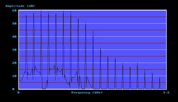
Figure 1. Anechoic Trumpet spectrum as originally derived by C P Boner
(first tone in the file below)

Recall that this is the acoustic spectrum of a pipe speaking in essentially anechoic conditions. This is important as far as this article is concerned, and it also makes Boner's data rather rare and therefore precious. Another factor is worth noting, concerning the relatively smooth spectral envelope (the curve obtained by joining up the harmonic peaks). When spectra are examined from pipes speaking in a room, that is in a non-anechoic environment, their spectra almost always appear far more 'ragged' than in this example. This phenomenon occurs because room effects (modes and phase interference) distort the amplitudes of the harmonics which the pipe radiates, and we shall see some examples presently. It is like listening to the original anechoically-derived sound played through a set of multiple narrow-band filters, some of whose tuned frequencies might correspond by chance to those of particular harmonics whereas others might not.

Having thus established a source of anechoic Trumpet pipe sound, it was replayed into a room and picked up by a pair of reasonable-quality capacitor microphones (Behringer C-2) mounted 13 cm apart on a stereo bar. Only one loudspeaker was used, to simulate an organ pipe which emits sound as a monaural source from a single location. The loudspeaker was a high quality unit (a KEF Reference 104). The microphones did not face the loudspeaker but rather they were oriented along an axis 90 degrees away from it and facing the longer wall of the room. The room was rectangular and fairly small, cluttered with furniture and bookshelves and thickly carpeted. It is probably not unlike the 'dens' into which many digital organs and virtual pipe organs are often banished. Subjectively it was completely acoustically dry with no discernible reverberation, but this does not signify that it was anechoic. On the contrary, it possessed marked ambience characteristics as the following analysis will demonstrate.

A composite file was prepared consisting of three tones as below:

1. The original anechoic source signal as described above.
2. The signal from one of the microphones.
3. The signal from the other microphone.

Each tone lasts for ten seconds, separated from the next by three seconds of silence. Each is identical in both the left and right channels (i.e. monaural). Therefore the two microphone signals do not appear as a stereo recording because the object of the exercise is to demonstrate the marked variation in sound resulting from the small change (13 cm) in listening position between them. Ideally you should listen to the file using headphones so that you are exposed only to the spectral distortions resulting from my recording room. If you listen with loudspeakers in your own room you will get the double dose of ambience which is the subject of this article. However there is no reason why you should not subsequently listen using loudspeakers if you want to form a subjective impression of the differences between single and double ambience imposed on an anechoic source. (NB set the volume low on your system at first so that you do not expose your ears to an excessively loud sound).

   Trumpet tones

In what follows, the subjective remarks about what I hear when listening to this file might not coincide with your own impressions. It is worth bearing this in mind because people perceive sounds differently.

You might reflect on the fact that the first tone on this recording is substantially the same sound you would hear if you heard this Trumpet pipe speaking into an anechoic chamber, and not many people have had the opportunity to do that! So aren't you lucky? It is also probably the first time that the sound of Boner's Trumpet has been played to an audience in nearly eighty years, and of course he could not have actually recorded it himself at the time, at least not in high fidelity. The only recording means available to him was the then-expensive process of making a 78 rpm shellac phonograph record, complete with all the scratches, clicks, pops and hiss which that would have entailed. So all he could do was to present its frequency spectrum in his paper, which was shown earlier in Figure 1. Spectra of the two succeeding tones in the composite file, those from the two microphones in my listening room, are shown below in Figures 2 and 3: 

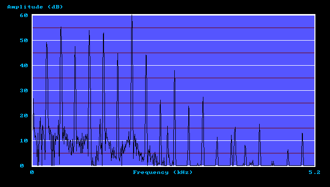
Figure 2. Trumpet spectrum received by microphone 1
(second tone in the file)

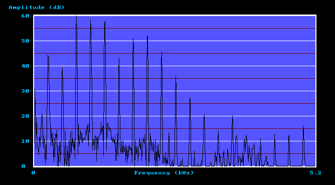
Figure 3. Trumpet spectrum received by microphone 2
(third tone in the file)

These two microphone spectra differ from the source spectrum (Figure 1) in three generic respects. Firstly there is more low-amplitude noise in the plots, and secondly some spectrum lines can be seen which are anharmonic (not harmonically related) in that they appear between pairs of true harmonics. Both these artefacts are due to low level background noise in the recording room, mainly due to computer fans, so they can be disregarded. Thirdly, the two microphone spectra are far more 'ragged' than the original for the reasons explained previously. Because the original anechoic spectrum envelope is so smooth it is easy to pick up the room distortions by eye (this was a major reason for using an anechoic source signal in the first place). Thus the three sounds in this composite file are clearly very different. The first tone in the file has the satisfying rounded sound one would expect of an American organ Trumpet pipe of this era (the 1930s). However that from microphone 1, the second tone in the recorded sequence, seems to have lost much of this. It sounds thinner, with the prominent seventh harmonic visible in the spectrum (Figure 2) being clearly audible. The signal from microphone 2, the third tone in the sequence, is decidedly odd. It does not sound like a Trumpet at all, having a third harmonic which seems to dominate the tone. Unsurprisingly, the spectrum (Figure 3) shows that this is the strongest harmonic. It is remarkable that such large differences occur between the signals picked up by two microphones only five inches apart, though such results are not unusual when dealing with room acoustics.

The differences were not the consequence of using a small recording room since dramatic changes occur over short distances in any non-anechoic listening space. The file below was recorded in the large reverberant volume of St George's church, Dunster in Somerset, England as the recording microphone was being moved around while a loud Trompette en Chamade pipe sounded. Just as in the experiment above, you can detect major tonal changes as the microphone moved through various regions of phase interference and different modes set up within the building:

   Signal from a moving microphone in a large church

What are we to make of this? Remember that we have not yet encountered the phenomenon of double ambience because all the tones so far have involved only a single room, provided you have been listening to them only with headphones. But before diving into that, we need to derive an Amplitude Transfer Function for the listening room we have just been discussing for reasons which will be described.

The Amplitude Transfer Function (ATF) of a room

Because we know the characteristics of the signal radiated from the loudspeaker and the signals received at the two microphones, we can derive information about the sound path between them. In particular it is helpful to know by how much an acoustic signal is attenuated as it travels from the loudspeaker to each microphone. This is called the Amplitude Transfer Function (ATF) of the room in this article. It is like an electronic attenuator whose attenuation can be defined once the input voltage (corresponding in this case to the sound pressure level radiated by the loudspeaker) and the output voltage (corresponding to the sound pressure level at the microphone) are known. Attenuation is the ratio of the output to the input voltages, and similarly the ATF is the ratio of the corresponding sound pressure levels. It is calculated at each harmonic frequency in the spectra shown earlier because it varies with frequency. Although the ATF therefore characterises the acoustic room response as a function of frequency, it only has meaning for the specific loudspeaker and microphone positions used in the experiment described earlier. Other positions would yield completely different results. It also only has meaning for the fundamental frequency of the tones used in the experiment, which was 261.6 Hz (middle C). The word 'amplitude' is used to emphasise that the ATF measurement refers only to the magnitudes of the oscillatory sound pressure levels, not their phases, because the ear is insensitive to phase.

We can consider the spectra shown previously to represent sound pressure levels radiated by the loudspeaker and received at each microphone, though not in an absolute sense. They only represent measurements relative to some arbitrary datum, therefore the vertical axes display sound pressure levels over a range of 60 dB (a ratio of 1000:1) without saying what the levels actually are in units such as Pascals. Also, because decibels have been used, we do not divide the values to get an ATF attenuation ratio but instead we subtract one from another. This is because decibels are logarithmic quantities - multiplication and division are replaced by addition and subtraction when logarithmic arithmetic is used.

Let us see how the ATF is derived for microphone number 1. The spectrum of the signal it received is at Figure 2, and the spectrum of the signal radiated by the loudspeaker is at Figure 1. For each harmonic we simply subtract its dB value in Figure 1 from the corresponding dB value in Figure 2. The set of 19 numbers so obtained is the ATF for microphone 1. Clarifying this with more detail, from Figure 2 the first few dB values of the microphone spectrum are 49, 55, 47, 53, ... etc and from Figure 1 the first few values of the spectrum radiated by the loudspeaker are 57, 59, 60, 59, ... etc. Subtracting the second set of numbers from the first gives the ATF for this microphone as -8, -4, -13, -6, ... etc. Similarly, for microphone 2 we subtract the dB values in Figure 1 from those in Figure 3, again for each harmonic, and we get another set of 19 numbers. These two sets of numbers measure the acoustic attenuation of the room between the loudspeaker and each microphone as a function of frequency, and they will be used presently when we look at the double-ambience situation.

All this assumes that the frequency responses of the loudspeaker and both microphones were flat in the approximate range from 250 Hz to 5 kHz over which the spectrum measurements were made. The loudspeaker was supplied with a calibration curve obtained in an anechoic chamber for that model and this showed deviations of only a few dB. The microphones were a matched pair with a sensitivity curve so suspiciously flat that it did not look as though it had been measured at all, let alone in an anechoic chamber. However even the cheapest capacitor microphone capsules (though these microphones were not particularly cheap) usually have a remarkably uniform frequency response over the entire audio range, their main shortcoming being an overall sensitivity variation as they age. This would not affect the results here. Consequently no frequency compensation was applied to account for the loudspeaker and microphone responses.

Double room ambience - a demonstration

Double ambience means that the original signal spectrum from an organ pipe is distorted twice, once by the room in which the pipe speaks and again by the different room which a digital organ occupies. This is because the samples in the digital organ's memory were recorded in the first room and then replayed in the second.

We cannot get at the original signal spectrum of the pipe unless it had been recorded anechoically beforehand, which is highly unlikely. However it is easy to obtain the distorted version at the microphone position in the room where the recordings were made. Just as in the examples shown earlier, such microphone spectra tend to be 'ragged', the raggedness representing mainly the distortion imposed by the recording room as we saw for the Trumpet spectra previously. Another example is shown below in Figure 4.

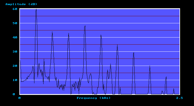
Figure 4. Middle C Great Open Diapason spectrum from a recording in St Mary Ponsbourne church (J W Walker 1858)
(first tone in the file below)

This shows the spectrum of the middle C Open Diapason pipe on the Great Organ of the historic Walker instrument of 1858 at St Mary Ponsbourne in Hertfordshire, England, and thanks are due to the organist of the church, Paul Minchinton, for making the recording. As the recording was made in the church it had already been distorted once by the acoustic properties of the building, which has made at least some of the harmonics jump up and down capriciously. In a general sense this behaviour mirrors that observed already with the Trumpet spectra which were also distorted once, but in the very different listening space of the smaller room already discussed. Now imagine this recorded Diapason waveform to be loaded into the memory of a digital organ which is then played in that small room. Its spectrum would be distorted again by that room as were the Trumpet spectra we saw earlier, so the signals would sound different to how they sounded in the original building, St Mary's church. However, this time we can predict accurately how this organ pipe will sound without having to go to the trouble of actually radiating its signal from a loudspeaker and picking it up with microphones. This is because we now have the two Amplitude Transfer Functions (ATFs) of the small room corresponding to the two previous microphone positions. By subtracting the two sets of attenuation values for each harmonic from the harmonic values in Figure 4, two new spectra will be obtained which are shown in Figure 5 and 6.

To clarify, the first few dB values in Figure 4 are 60, 43, 42, 48, ... etc and the ATF for microphone number 1 is -8, -4, -13, -6, ... etc. as discussed in the previous section. Therefore the new spectrum is obtained by adding these numbers (not subtracting, because the ATF is already negative), giving 52, 39, 29, 42, ... etc. As a final step this resulting spectrum is normalised so that its largest harmonic becomes 60 dB, which means adding 8 to the values just derived. This does nothing to the tone quality as it merely increases the volume of the signal. Thus the final numbers are 60, 47, 37, 50, ... etc. This spectrum is plotted in Figure 5. (Some of the data points in all of these graphs might not coincide exactly with the calculated values because of rounding and truncation in the plotting algorithm used).

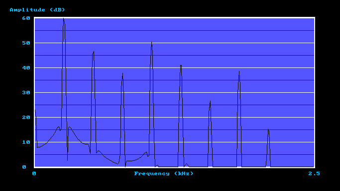
Figure 5. Calculated Open Diapason spectrum at the microphone 1 position
(second tone in the file)

The spectrum for microphone 2 is calculated in exactly the same way except that the other ATF is used. This spectrum is shown in Figure 6.

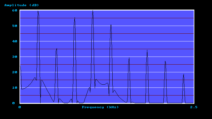
Figure 6. Calculated Open Diapason spectrum at the microphone 2 position
(third tone in the file)

These three graphs are obviously different to each other, just as the Trumpet spectra were previously. But it is more important what the ear makes of the sounds. So as before, a composite file was prepared consisting of the three tones below, which you should listen to using headphones to avoid muddying the waters by adding the ambience of yet another room (your own) to the mix:

1. The original Open Diapason recorded in the first room (spectrum in Figure 4).
2. The calculated waveform at the position of microphone 1 in the second room (spectrum in Figure 5).
3. The calculated waveform at the position of microphone 2 in the second room (spectrum in Figure 6).

The two calculated waveforms were derived by applying additive synthesis to the harmonic amplitudes in the corresponding spectra. Only the steady-state sounds are heard to avoid distracting the ear by retaining artefacts such as attack transients.

   Open Diapason tones

The first tone corresponds to that recorded in St Mary's church (the first room) so it was only distorted once by the ambience of the building. However the two succeeding tones have been distorted again by the additional ambience of the second, smaller room. This second dose of ambience was captured within the two Amplitude Transfer Functions which were impressed on the original signal. To my ears the second tone is not very different from the first, but the third is totally unlike the original. Yet these latter two tones represent listening positions in the second room separated by only five inches, which was the separation between the microphone positions for which the ATFs were calculated.

 
So this demonstration of double ambience has shown why a digital organ can sound grossly different to the pipe organ whose tones reside in its memory. On the basis of the foregoing it is difficult to deny that the effect exists and that it is potentially a major one. It illustrates the magnitude of the double ambience problem.

But all this begs the question as to how the ear and brain can somehow make sense of the distortions imposed by room ambience. In some way we seem to be able to 'listen through' these distortions to form a meaningful impression of the quality of an organ in a building. Of course, this statement relates to just a single dose of ambience when listening to an organ in the building itself. Whether we have as good a capability to 'listen through' the two stages of distortion implied by double ambience is a different matter, and I would argue that at least some of us might not have such a capability. My reasoning for saying this is that our auditory apparatus presumably learns to accept a single dose of room ambience with its inherent spectral distortions because we grow up with it from our earliest days. Thus in some way perhaps we develop an unconscious ability to compensate for what rooms do to sounds. However this does not imply that we can also compensate for double ambience, which is effectively two rooms in series.

 
It is possible that our brains average out the distortions which a room imposes on a spectrum. This is because our ears are not fixed rigidly in position like a pair of microphones but instead they are free to move around, even if we sit still and just move our heads slightly. The extreme sensitivity of distortion to listening position was illustrated by the signals presented earlier corresponding to microphone positions only a few inches apart, which happens to be comparable to the separation between our two ears. Because we listen binaurally, the brain might also average the spectra received by each ear in addition to real time averaging during movement. However averaging could not compensate fully for the distortion due to double ambience because no amount of movement in the listening room could affect the fixed microphone position in the recording room. Double ambience is a wholly artificial listening environment which never arose in human experience until the advent of audio broadcasts and recorded sound. Consequently it would unsurprising if our brains have not evolved with the ability to fully process sounds which come to us via two stages of ambience. If so, then maybe this is one reason why some people find sampled-sound digital synthesis inherently unsatisfactory and why they can readily identify digital organs as those which do not use pipes.

Concluding remarks

Sampled sound synthesis is used widely in digital organs and universally in virtual pipe organs. Usually the samples are recordings of actual organ pipes, therefore manufacturers frequently claim that their products sound indistinguishable from the real thing. However the article has showed that this claim is questionable for at least one reason - double ambience. This term reflects the fact that the recordings are made in one room whereas the instruments are played in another. It is well known that room ambience imposes often gross distortions on the harmonic amplitudes which constitute the frequency spectrum of an organ pipe, and it was shown that the distortion varies dramatically over distances of a few centimetres. Therefore when the ambiences of two rooms effectively in series are involved, the already-distorted waveforms in the memory of a digital organ will be distorted in a different way for a second time when the instrument is played. Aural examples of the effects of single and double ambience on reed and diapason tones were presented to illustrate the problem.

It is likely that the brain can compensate to some extent for the ambience of a single room using mechanisms such as real time averaging during head and body movements. However this will be less effective when double ambience is present because no amount of movement in the listening room can compensate for the fixed microphone position in the recording room. Double ambience is in fact a wholly artificial listening environment which never arose in human experience until the advent of broadcast audio and recorded sound. Consequently it would unsurprising if our brains have not evolved with the ability to fully process sounds which come to us via two stages of ambience. If so, then maybe this is one reason why some people find sampled-sound digital synthesis inherently unsatisfactory and why they can readily identify digital organs as those which do not use pipes.

Appendix 1 - The technical quality of Boner's results

The essentials of Boner's experiments were that nearly-anechoic acoustic measurements were made of organ pipes mounted on a tower 24 feet (7.3m) above the ground out of doors. Their sounds were picked up by a ribbon microphone at the same height and spectrum-analysed using a type 636-A wave analyser made by the General Radio Company. Astonishingly, it is still quite easy to find the instruction manual and detailed schematics for this obviously well-known instrument on the internet [4], and from this one can glean a lot of useful information. Thus we find that the 636-A was an early example of a line of functionally similar test gear marketed subsequently by many firms worldwide for several decades. It consisted of a very narrow band filter which was scanned manually across the desired frequency range while the pipe under test sounded continuously. The harmonic amplitudes emitted by the pipe were obtained by noting down the peak readings from a voltmeter incorporated in the instrument. The analyser used a heterodyne technique and a fixed-frequency quartz crystal filter to achieve the narrow analysis bandwidth, rather than the impractical alternative of a directly-variable analogue filter.

Although there was nothing wrong in principle with this idea the user manual shows that there were some practical downsides, not the least of these being the need to frequently re-calibrate the instrument especially as it apparently ran on battery power. In those early days of thermionic electronics the calibration instability is not surprising. However one can presumably take for granted that this would have been taken care of in the careful professional environment of a university physics laboratory by one who was prepared to put his name to a published paper in a respected journal. Moreover the 60 dB dynamic range achieved within the narrow filter bandwidth, as evidenced by the published acoustic spectra, is what one could reasonably have expected from analogue instrumentation of the day. If there was a limitation in this regard it would more likely have arisen from interfering ambient noise in the outdoor measuring environment rather than from deficiencies in the test gear. But the killer statement in the paper which largely lays one's concerns to rest is that which says "readings on the same pipe on several days checked to within 3 dB, provided wind pressure and tuning remained constant". So we are probably safe to assume that Boner's results obtained in near-anechoic conditions are sufficiently robust to warrant attention today. They remain important in view of the absence of a comparable body of anechoically-derived data elsewhere in the public domain.

References

1. "Equalising Loudspeaker Sensitivities", an article on this website, C E Pykett, 2012

2. "Acoustic Spectra of Organ Pipes", C P Boner, J Ac Soc Am, (10), pp. 32 - 40, July 1938

3. See www.hammondclub.nl/nl/menu/Hammond/Laurens-Hammond/De-Hammond-rechtzaak--Eng (accessed 20 March 2017)

4. See www.ietlabs.com/pdf/Manuals/GR/636-A%20Wave%20Analyzer.pdf (accessed 20 March 2017)