


|
|
|
Waveforms and Spectra - or - Amplitude and Phase
by Colin Pykett
... don't take any notice, it's just a phase ...
Posted: 29 December 2013 Revised: 29 December 2013 Copyright © C E Pykett 2013
Abstract. Using both visual and aural examples, this article shows that the organ pipe waveforms we can view on an oscilloscope screen or a wave editor are the result of adding all the harmonics together, taking account of not only the amplitude of each harmonic but its phase as well. However, because the ear is insensitive to phase, it is only the harmonic amplitudes which are important to our perception of timbre or tone quality while the pipe sounds in its sustained or steady-state speaking regime. Therefore the phases can be adjusted at will without modifying tone colour. This can be useful if a waveform has a high crest (peak) factor which results in the available signal headroom in a synthesiser being used inefficiently. Such waveforms suffer from subjective loudness and signal to noise ratio limitations which might be less than optimum. It is shown that the crest factor can be reduced by adjusting the relative phases of the harmonics. It is also pointed out that spectrum analysis can be applied to audio signals using Fourier transforms which are only half as long as those used traditionally, because the phase information present in the source waveform can be discarded. This results in useful improvements in both memory size and execution speed in some music applications.
Contents (click on the headings below to access the desired sections)
Harmonic amplitudes and amplitude spectra
Harmonic phases and phase spectra
It is a tantalising truism that if we can reproduce exactly (at our ear drums) the waveform of an organ pipe as it sounds in the building housing the instrument, then we will be unable to distinguish between the original and the reproduced sounds. This is one reason why the majority of digital organs still use sampled sound synthesis today, even though alternative methods such as FM, additive, subtractive and physical modelling synthesis still exist or have been tried. In sampled sound synthesis the sounds of actual organ pipes are first recorded, then captured in a computer memory, and finally recalled on demand as the simulated instrument is played.
However it is less well known that, with sampled sounds, it is also true that the two waveforms - the original and its reproduction - do not need to be identical. In fact, under certain conditions they can differ dramatically in appearance if viewed on an oscilloscope screen or in a wave editor, yet the ear will not be able to detect the difference. Although the reasons for this are straightforward, they do not seem to be universally understood, judging from my email inbox and chatter on discussion forums, so this article tries to explain how the apparent paradox arises.
Harmonic amplitudes and amplitude spectra
First let us recall that the waveform of any organ pipe while it sounds continuously is made up from a number of harmonics. We refer to a plot of the amplitude of each harmonic versus its frequency as the amplitude spectrum (also called the power spectrum) of that pipe sound, and an example is shown below in Figure 1. This is the spectrum of an actual Cornopean reed pipe while it was sounding in its sustained or steady-state speaking regime after the attack transient had died away..
Figure 1. Amplitude spectrum of a Cornopean organ pipe
In this case there are nearly 20 harmonics including the fundamental or first harmonic, each one of which is a sine wave at a different frequency. The frequencies are integer (whole number) multiples of the fundamental frequency, which in this case was 370 Hz corresponding to the F sharp above middle C. Thus the harmonic frequencies are 370 Hz (the fundamental), 740 Hz (370 times 2), 1110 Hz (370 times 3), 1480 Hz (370 times 4), and so on. If we generated all these sine waves separately with the correct amplitudes as shown by the spectrum, and then added them together by playing them simultaneously, we would hear a sound identical to that of the original Cornopean pipe. This process is additive synthesis, which was used in the Bradford computing organ developed back in the 1980s. However, the interesting aspect is that the waveform when synthesised additively in this way will often not look at all like the original waveform of the Cornopean pipe when it was recorded. So how, then, can the two waveforms sound the same?
Harmonic phases and phase spectra
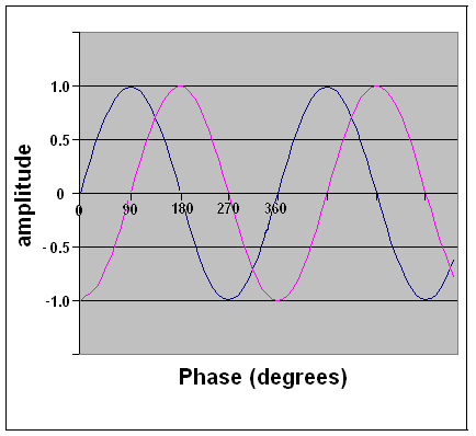
The resolution of the paradox lies in the relative phases of the various harmonics. Each harmonic in the original sound is a sine wave having a particular frequency, and any sine wave has not only a frequency and an amplitude (its height when viewed on an oscilloscope) but a phase as well. The phase of a harmonic indicates by how much it is shifted or slid along the horizontal (time) axis relative to the others. Phase is measured as an angle, with 360 degrees representing a complete cycle of the sine wave. This is illustrated in Figure 2 below.
Figure 2. Two sine waves of equal amplitude and frequency but with a 90 degree relative phase shift
Thus to shift the phase of any harmonic by up to one cycle, one adds or subtracts any number between 0 and 360 degrees to its original value. Therefore there is also a phase spectrum for an organ pipe sound as well as an amplitude spectrum, the phase spectrum being a graph indicating how the phase of the waveform varies with frequency. Phase spectra are seldom discussed in audio work though, which is why I have laboured the topic somewhat here. However the point is that, unless these harmonic phases of the original sound are measured and then applied to the resynthesised sound, harmonic by harmonic, the resynthesised waveform will look different. This is because an arbitrary phase, often zero, is usually applied to each harmonic when performing additive synthesis by computer. The shape of the synthesised wave depends not only on the amplitudes of the harmonics it contains but also on their phases.
Why can this apparently drastic step be taken to fiddle around with the harmonic phases in so capricious a manner when performing additive synthesis? Simply because the ear and brain are insensitive to the relative phases of the harmonics - only their relative amplitudes are used by our neural processing to derive the characteristics of the sounds we perceive consciously [5]. It is reasonable to conclude that the relative phases among the various harmonics of the sounds occurring in nature are presumably not very important to survival, because our auditory systems have obviously evolved to ignore them. When we do a frequency analysis of a waveform the phases can be computed from the original recording just as easily as the amplitudes, in fact they are generally (but not always) available as a by-product of the Fast Fourier Transform (FFT), but the phase information is discarded deliberately when deriving an amplitude spectrum such as that in Figure 1.
To help understand why adjusting the phases of the harmonics can result in dramatic changes to the shape of a waveform, let us look at a much simpler example of a sound which contains only two harmonics. I constructed two waveforms, both comprising sine waves at 440 Hz and 880 Hz which were added together. These frequencies represent the fundamental and second harmonic of a composite waveform whose pitch is the A above middle C. Both of these composite waveforms were identical except that in one case the phase difference between the two harmonics was zero, and in the other case the phase difference was 90 degrees. A few cycles of both of these composite waveforms are shown in Figures 3 and 4.
Figure 3. Waveform consisting of two harmonics with a relative phase of zero.
Figure 4. Waveform consisting of two harmonics with a relative phase of 90 degrees.
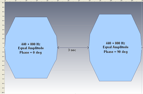
It is obvious that the two waves are different, yet they sound identical. You do not have to take my word for it because I have prepared a short audio clip which contains both waveforms played one after the other. So that you will know what to listen for, Figure 5 shows the basic structure of the clip. The first few seconds consists of the two harmonics with zero phase shift. There is then a short gap before the second composite wave is heard in which the phase shift is 90 degrees. If you can perceive a subjective difference between the two I would eat my hat - if I wore one.
Figure 5. Amplitude envelope of the aural demonstration clip
Here is the sound clip:
I can hear some of you beginning to murmur things like "so what?" The majority of the article so far has been to do with additive synthesis, a technique which is now vanishing from the digital organ scene, so how is it relevant to sampled sound synthesis? If we can capture and reproduce sounds so successfully with a sampled sound synthesiser, which we can, why should we bother about the minutiae of an alternative technique which is disappearing rapidly?
The question is valid, but only in those cases where one can record high quality samples to start with. In other words, one can only generate a sample set in the usual manner if the original pipe organ exists and is in sufficiently good condition. Although merely a statement of the blindingly obvious, it is nevertheless a big drawback of sampled sound synthesis as currently practised. This is because sometimes one might wish to build a sample set from an important or otherwise interesting organ whose pipework is in a parlous state. Or one might wish to re-create from scratch an approximation to the sounds of an organ that had long vanished. In neither case could samples be recorded in the usual way. I have addressed this problem in detail and have created sample sets for a number of instruments which no longer exist or which are otherwise inaccessible, and my approach is described elsewhere on this website in reference [1]. As part and parcel of generating the sample sets in these cases I have often had recourse to additive synthesis. For instance, one can create a clean, noise-free sample to simulate a particular pipe using off-line additive synthesis, using a noisy recording or an off-speech pipe as source material. One can also synthesise and then add attack and release transients to it. Yet another opportunity for using such techniques arises if one only has a sparse, incomplete sample set for a particular organ, and in this case it is necessary to fill in the missing notes by creating new samples for them using nearby samples as 'voicing points'. I have described this approach in detail in reference [2]. In some of these situations it is necessary to pay heed to the phase spectra of the additively-synthesised waveforms, especially if one is trying to join other wave segments such as transients onto them. Any discontinuities between the harmonic phases in the transient and steady-state parts of the waveforms will be painfully obvious unless they are remedied.
So far I hope this article has been relatively easy to comprehend. However it is perhaps surprising how many fascinating twists and turns we encounter when we follow the route signposted "phase", particularly as it is a subject seldom discussed in digital music. Consequently this section introduces a couple of further aspects which are probably of most interest to those more immersed in the technical background to digital sound synthesis.
Although it is possible to do additive synthesis by simply assigning a phase value of zero to each harmonic, and this is often done, advantages can be gained if one proceeds in a somewhat smarter manner to generate a better phase spectrum.
A problem arises if the same phase angle (zero or any other value) is assigned to all the harmonics prior to performing additive synthesis. It occurs because at some point in each cycle of the synthesised waveform all the harmonics will be rising or falling simultaneously, and because they are being added together, this can result in a big positive or negative spike which has a much larger amplitude than the remainder of the waveform. If a zero phase angle is used, this spike occurs at the beginning of the waveform and thereafter at the beginning of each subsequent cycle. An example is shown in Figure 6.
Figure 6. Additive synthesis applied to 5 harmonics with zero phase
This shows two cycles of the waveform resulting from adding five harmonics together with phases equal to zero. The large spikes at the start of each cycle, referred to above, are clearly visible. Such high crest factor waveforms are undesirable because they make inefficient use of the headroom available in any processing system, be it analogue or digital. Away from the peaks, and therefore for most of the time, the amplitude excursions are only utilising a fraction of the maximum bit depth in a digital system for example, because the short-duration spikes also have to be accommodated without clipping. This means that quantisation noise is higher over most of the waveform than it need be were the waveform a better-behaved one in which the spikes were suppressed.
This desirable state can be approached by assigning a different phase to each harmonic, resulting in the waveform shown in Figure 7.
Figure 7. Additive synthesis applied to 5 harmonics with phase optimisation
In this case the different phases have resulted in the former large spikes becoming significantly smaller. The timbre or tone quality of the wave still sounds the same as before because the ear does not care about phase, but because we can now turn up the volume before clipping occurs, the sound is louder. More to the point, the signal to noise ratio has been improved.
Similar issues can arise when using physical modelling synthesis if the model results in a high crest factor waveform being generated. In these cases the same advantages can be gained by refining the model so it optimises the phases of the harmonics.
An effective automatic phase optimisation algorithm was first described by Schroeder [3] in the context of radar and sonar signal design, a field in which I used to work. In radar, sonar and also in digital audio, the phase to be applied to each harmonic (the phase spectrum) is necessarily specific to each waveform because there is no general solution to the problem. Thus Schroeder's algorithm generates a bespoke phase spectrum for a given signal which yields a low peak factor, often comparable to that of a sine wave of equal signal power. In general the high crest factor problem gets worse as the number of harmonics gets larger. Only five were present in the example just discussed, whereas a signal containing 31 harmonics was examined in Schroeder's paper. Illustrations analogous to those above for this signal are shown in Figures 8 and 9.
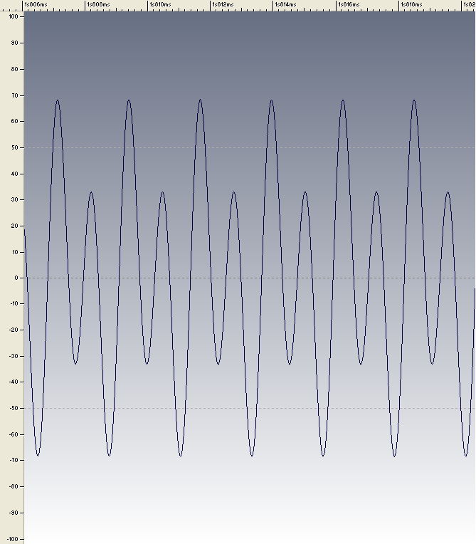
Figure 8. Two cycles of a signal synthesised from 31 harmonics with equal (zero) phase after Schroeder [3]
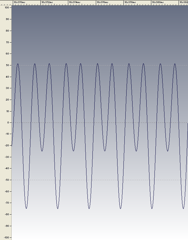
Figure 9. Two cycles of a signal having the same amplitude spectrum as Figure 8, synthesised from 31 harmonics using Schroeder's phase optimisation algorithm after Schroeder [3]
The very high crest factor of the synthesised waveform when all harmonics have the same phase can be seen from Figure 8, while the effectiveness of Schroeder's algorithm is apparent from the phase-adjusted harmonics in Figure 9. The amplitude scale of both graphs is the same, and it can be seen how the peaks have been completely removed. Such a signal utilises the available headroom in any processing system far more effectively than does one with a high crest factor. If these two waveforms represented an audio signal, they would sound exactly the same as far as their tone colours were concerned, even though they look completely different. Only their phase spectra differ, and we have noted several times that the ear is insensitive to the relative phases between the harmonics.
Similar waveforms to those above arise when simulating organ pipe sounds. The lower notes of a reed stop, for instance, frequently have a very large number of harmonics, often far more than the 31 used in Schroeder's example. Moreover, they often have amplitudes which only fall off gradually, thus many harmonics of significant amplitude are able to contribute to the formation of a large spike once per cycle.
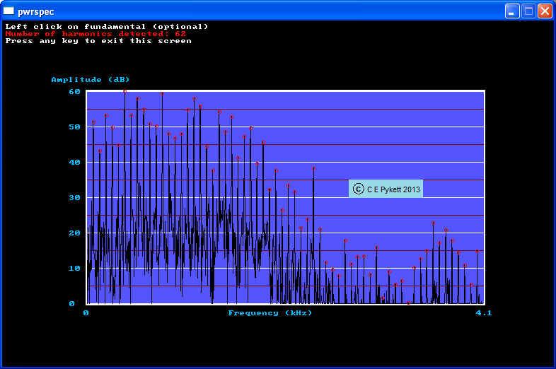
Figure 10. Amplitude spectrum of bottom C of an 8 foot Trompette stop
Both these attributes are evident in Figure 10, which is the amplitude spectrum of the bottom note of an 8 foot Trompette stop on a French organ. The number of harmonics in the plot is 62 (they are identified by the small red circles to differentiate them from noise spikes), and their amplitudes only begin to fall off significantly after the 30th or so. Such a spectrum would result in a high crest factor were it used to synthesis a waveform additively without adjusting the phases of the harmonics. Reducing the crest factor can increase the loudness of the sound in a sampled sound synthesiser without increasing the gain downstream of the rendering engine, which is the same thing as saying that the signal to noise ratio is enhanced. This occurs because the signal power of the waveform imported into the synthesiser is greater if its crest factor is low than if it were high, assuming that the peak signal amplitude was the same in both cases.
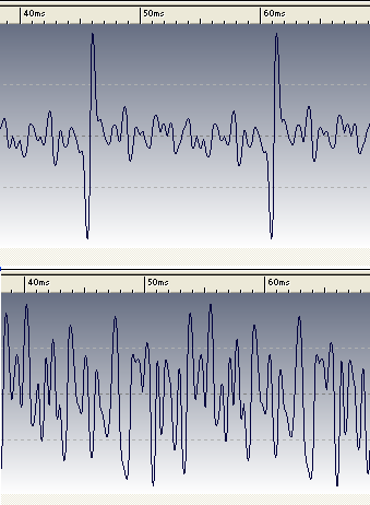
Figure 11. Waveforms of bottom C of an 8 foot Trompette stop - (upper) all harmonics have the same phase; (lower) harmonic phases were adjusted for a low crest factor
The points made above regarding the waveforms synthesised additively from the spectrum shown in Figure 10 are illustrated in Figure 11. Without adjusting the phases of the harmonics the high crest factor which results is shown in the upper picture, whereas when the phases are so adjusted the crest factor reduction is obvious from the lower. Both pictures have the same amplitude scale.
Both these waveforms can be auditioned from the sound clip above (the high crest factor wave plays first, the low crest factor one second). The low crest factor wave is noticeably louder even though the peak signal amplitudes were the same in both cases. This difference is easily detectable on the single notes comprising the clip, and therefore when chords are played the loudness increase can be spectacular. Note, yet again, that the considerable visible differences between these two waveforms do not affect the subjective tone colour of the sound (but see note [6]).
When doing additive synthesis it is often necessary to first analyse the frequency structure of a source waveform to enable its amplitude spectrum to be obtained. The number of harmonics and their amplitudes can then be derived from such a spectrum, which are input as data to the additive synthesiser. Normally the FFT (Fast Fourier Transform) algorithm is used to compute the spectrum, and traditionally this requires a transform of size N to handle N data values. (N is often restricted to an integer power of two, such as 1024, 2048, etc). However the FFT actually manipulates complex numbers which have both a real and an imaginary part, and the amplitudes and phases of the harmonics are extracted from the complex numbers which result from doing the transform. However, if we are not interested in the phases of the harmonics in the source data, and in digital audio we usually are not, we can take advantage of the fact that the input waveform to the FFT can then be regarded as a sequence of real, not complex, data values. Therefore we can use a variant of the FFT algorithm which only requires a complex transform of size N/2 to handle N real data values. Singleton's algorithm was one of the first to exploit this considerable simplification [4]. His paper also described a mixed-radix FFT in which N is not restricted to a power of 2. Both of these are important in some real-time music applications because of the memory size and execution speed improvements which result.
It has been shown using both visual and aural examples that the organ pipe waveforms we can view on an oscilloscope screen or a wave editor are the result of adding all the harmonics together, taking account not only of the amplitude of each harmonic but its phase as well. However, because the ear is insensitive to phase, it is only the harmonic amplitudes which are important to our perception of timbre or tone quality while the pipe sounds in its sustained or steady-state speaking regime. Therefore the phases can be adjusted at will without modifying tone colour. This can be useful if a waveform has a high crest (peak) factor which results in the available signal headroom in a synthesiser being used inefficiently. Such waveforms suffer from subjective loudness and signal to noise ratio limitations which might be less than optimum. It was shown that the crest factor can be reduced by adjusting the relative phases of the harmonics.
It was also pointed out that spectrum analysis can be applied to audio signals using Fourier transforms which are only half as long as those used traditionally, because the phase information present in the source waveform can be discarded. This results in useful improvements in both memory size and execution speed in some music applications.
1. "Re-creating Vanished Organs" , an article on this website, C E Pykett, 2005.
2. "Creating Sample Sets for Digital Organs from Sparse Data" , an article on this website, C E Pykett, 2013.
3. "Synthesis of Low-Peak-Factor Signals and Binary Sequences With Low Autocorrelation", M R Schroeder, IEEE Transactions on Information Theory, January 1970, p. 85.
4. "An Algorithm for Computing the Mixed Radix Fast Fourier Transform", R C Singleton, IEEE Transactions on Audio and Electroacoustics, June 1969, p. 93.
5. The ear is insensitive to the phase spectrum of a sound provided the phases remain constant, that is, they do not change with time. If they do change, then the ear will in general perceive the fact. The reason is that phase changes alter the frequencies present in the sound while the phase is in the process of changing, because frequency is proportional to the rate of change of phase. However the relative phases of the harmonics during the steady-state sounding regime of an organ pipe do not change substantially, any more than their relative amplitudes do. If they did, the resulting waveform would not be periodic and it would not sound like a real organ pipe.
6. It is best to play these two audio examples as nearly as possible at same subjective loudness by quickly adjusting the volume control of your audio setup before the second one is heard. This is because perceived tone colour is slightly dependent on loudness for some people. There may also be an issue owing to the use of MP3 encoding to reduce the file size here. The statement in the main text that the two waveforms sound the same applied to the original WAV (PCM) file before it was converted to MP3 format. Although MP3 decoding is tightly defined, there can be no guarantee that any particular decoder (such as the one you are using) complies with the standard. Moreover, the MP3 encoding process is only loosely defined. The MP3 encoder I used was part of Steinberg's WaveLab package, but I have no idea what it actually does. There is also a body of opinion which suggests that MP3 codecs do not cope well with high crest factor (peaky or impulsive) waveforms. Therefore, for these reasons I cannot predict what you might hear when you replay this file.
|