


|
|
|
Music based on natural electromagnetic phenomena
Colin Pykett
"Nature has conveniently tuned her first Schumann mode to 64 foot C"
Posted:
13 November 2020
Contents
Introduction
From the moment we are born we are immersed in a cauldron of Nature's sounds. Obvious examples are those made by the weather, such as the wind blowing through trees. Another is thunder, and the lightning which causes it also generates electromagnetic (radio) waves as well as sounds. But unlike thunder, the radio waves cannot be heard directly since their presence can only be revealed by using a suitable receiver. However a lightning receiver can be very simple, consisting essentially of a vertical rod aerial or antenna connected to an audio amplifier, and from its loudspeaker one can then hear a range of remarkable sounds having a natural musicality. The simplicity is made possible because the majority of the radio energy from lightning already lies in the audio frequency range, unlike manmade radio transmissions which use very much higher frequencies as carrier waves on which audio information is encoded. Because one does not need sophisticated equipment to hear the sounds of lightning it has become a thriving hobby [1], a particular fascination being the range of sounds picked up. Besides the predictable clicks and crackles of the lightning bolts themselves are other, quasi-musical, sounds with descriptive names such as whistlers, chorus and tweeks. These have inspired a lot of music, and several websites exist containing examples of the sounds themselves as well as some of the music [2].
However the story does not stop here. Besides generating audio frequency radio waves, lightning is also responsible for energy at much lower frequencies in the infrasonic region below the limit of human hearing (about 15 Hz), but remember that the energy we are speaking of is still electromagnetic rather than acoustic in origin. As we descend into this region we first encounter what are called Schumann resonances. Briefly, they arise within the thin spherical shell, shaped like an orange peel, lying between the earth's surface and the reflective ionosphere about 50 km (30 miles) above it. This shell acts as a cavity resonator for the radio waves radiated by lightning, and the fundamental resonant frequency of the cavity is about 8 Hz with a retinue of partials above this figure. So with a suitable receiver we could, in theory, listen to Schumann resonances just as we can for the other sounds of lightning such as whistlers. However it would require a loudspeaker system of gargantuan proportions before we could begin to feel, rather than hear, such low frequencies as infrasound. Nevertheless it would be possible to do it, and in the organ world some large instruments have been made whose longest pipes generate 8 Hz (64 foot C) used in pedal stops with fearsome names such as Gravissima [3]. Also the use of rhythmic, harmonic and melodic constructs inspired by the Schumann frequencies, rather than the infrasound itself, is popular in New Age music intended for relaxation and healing purposes, the association with the 'sounds of the earth' allegedly augmenting the effects psychologically if not mystically.
This article contemplates the possibilities for creating music based on the infrasonic Schumann resonances and on ULF waves below 1 Hz. Other sounds of lightning such as whistlers are not discussed further as these, being relatively easy to detect and already in the audio range, have been used by musicians for a long time. However all of them share the common fascination that they have always been part of the environment in which we live. All of them can justifiably be regarded as the Music of the Spheres or the Sounds of the Cosmos, and therein lies their attraction. Some audio examples are included in the article to demonstrate the wide range of novel sounds which can be rendered digitally and hence used in music. At that point the topic then becomes limited only by the imagination of the composer and performer, so the purpose of this article is to highlight the basic ingredients which they can manipulate rather than to present fully worked up compositions.
Lightning or church bells? - Schumann resonances
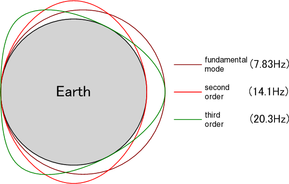
We now start to look at the topics outlined above in more detail, and the first is Schumann resonances. As mentioned already, these arise from lightning discharges within the thin spherical cavity or shell between the earth and the ionosphere. 'Resonances' is used in the plural because the fundamental frequency at about 8 Hz exists together with several inharmonic partials lying above it. Using the terminology rigorously, the partials are indeed partials rather than harmonics because their frequencies are not exact whole-number multiples of the fundamental. This results from the cavity having several peculiar properties we shall not go into. The first three Schumann partials are sketched in Figure 1 where they are denoted by the more usual term 'modes'. This usage is the same as that employed when speaking of the resonant frequencies of rooms for sound waves, which are also called modes. The electromagnetic energy from the lightning is confined within the cavity owing to the reflections it encounters at the earth's surface and at the ionosphere some 30 miles above it, thus it bounces around continuously within this space.
Figure 1. Illustrating the first three Schumann resonance modes [4]
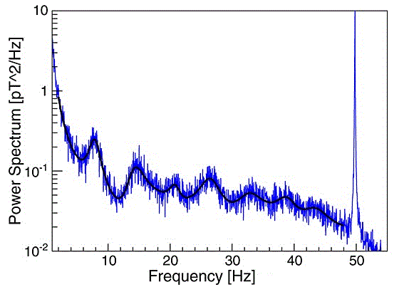
So the earth-ionosphere cavity forms a waveguide which 'rings' at all the Schumann mode frequencies simultaneously whenever a lighting bolt occurs anywhere within it. Because lightning strikes many times every second across the earth, the cavity is excited continuously although rather 'lumpily' in that particularly powerful discharges cause spikes in the resonance amplitudes. Thus there is a continuous musical humming sound all around us if we have the right sort of radio receiver to enable us to hear it. A typical frequency spectrum of an actual Schumann resonance signal from such a receiver is shown in Figure 2, though the frequencies and strengths of each partial can vary slightly at different times.
Figure 2. Typical frequency spectrum of Schumann resonances (Dyrda et al [5])
The 'grassy' blue trace is the spectrum of the raw data as recorded from the receiver, with the black curve indicating the best fit to it. The grass partly reflects fluctuations in the lightning events exciting the cavity, but it also reflects the very low strength of the wanted signal. Thus background noise is a major problem in detecting Schumann signals. Another manifestation of noise is the prominent power line spike at 50 Hz which is almost impossible to eliminate completely when an amplifier with such high gain has to be used to detect the signals in the first place. About six Schumann modes can be discerned starting near 8 Hz.
Owing to the poor signal to noise ratio it is pointless trying to use real Schumann data for musical purposes since the ear is swamped by the loud background mush plus the even more dominant 50 Hz buzz. Although the latter can be substantially reduced using offline noise reduction techniques when generating digital samples, these work less well on the mush because its statistical properties are non-stationary. This reflects the 'lumpiness' of the signal remarked on earlier. And any self-respecting musician would reject sound samples with the slightest vestige of mains hum especially since the desired higher-order Schumann modes lie so close to 50 Hz. Therefore I used synthetic data here, and when generating it I became aware of a rather remarkable coincidence. Defining the pitch standard of the data as A440, the frequency of the first Schumann mode then turns out to be 8.2 Hz which is within the range encountered in practice [6]. Put another way, Nature has conveniently tuned her first Schumann mode to 64 foot C! It is also a happy coincidence from a musical point of view that one by the name of Schumann predicted their existence.
The synthetic sounds were generated by real time additive synthesis using six sine wave partials tuned to the mode frequencies shown in Table 1, with their relative amplitudes suggested by the spectrum in Figure 2. Thus each note keyed resulted in a polyphony demand of 6 in the synthesiser. Suitable attack and decay envelopes were added to each partial, and each was looped independently so that notes could be sustained indefinitely [7]. The key compass synthesised was 8 chromatic octaves starting at 64 foot C (MIDI Note Number 0).
Table 1. Mode frequencies and relative powers for the synthesised Schumann samples
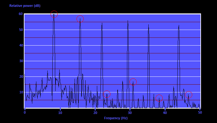
The measured spectrum of the synthesised waveform is shown in Figure 3, whence it can be seen that the signal to noise ratio is much higher than for the real data (Figure 2) and that the relative partial powers have been preserved.
Figure 3. Measured frequency spectrum of the synthesised Schumann resonances
The app used to compute this spectrum attempted to discover exact harmonics associated with the dominant first mode. Had they been present, they would have occupied the frequency slots identified by the red circles. As it is, the circles show that the second mode is nearly harmonic to the first, thus it is almost an octave higher, whereas subsequent ones are substantially flatter (lower in frequency) than true harmonics would have been. Therefore the harmonic identification algorithm was merely seizing on low level peaks of no significance in these cases.
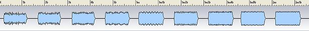
Sound files are now offered to give a flavour of what Schumann resonances sound like. The first clip is a sequence of nine notes at octave intervals starting at 64 foot C. Each note lasts for 10 seconds with a 5 second gap between adjacent ones. This simple file structure is shown pictorially at Figure 4 since it is important to know what to expect when you listen to it for the reasons below.
Figure 4. Structure of the synthetic Schumann sound file below
When listening for the first time it is VITAL to keep the volume low on your audio setup. The first sample at 64 foot C begins after a few seconds of silence. Be aware that it contains high-level infrasound at 8.2 Hz. Although the higher modes are at higher frequencies it is nevertheless quite possible that you might not hear very much, so you might be tempted to crank up the volume too far. However infrasound power at some level will probably be there in your listening space, and the better your system the more of it you will experience, so it could quite easily cause damage. Consequently it would be a good idea to observe or touch the woofer/subwoofer loudspeaker cones to ensure they are not being overdriven. Another reason for caution is because the wellbeing of some people is thought to be negatively affected by infrasound.
Here is the file:
Synthesised Schumann resonances 2m 16s/ 2.1 MB
The clip demonstrates the dramatic changes in subjective timbre or tone colour experienced over a frequency range of 8 octaves for a waveform whose partial structure is invariant. You will no doubt form your own impressions, but of particular interest is the emergence of a distinctly bell-like quality around middle C. Elaborating on this discovery, the file below is of a typical bell or chime sequence played in the octave from middle C to treble C:
Synthesised Schumann resonances - 'bell' sounds 17s/ 274 kB
Observe that we are now using the timbral structure of naturally-occurring infrasound to make audible music, which is the whole point of this article even though it has taken a long time to get here. So congratulations to those who have persevered this far! To emphasise the bell-like quality, Table 2 compares the partial frequencies of the Schumann modes used in this article to those of bells.
Table 2. Partial frequencies of typical Schumann signals and bells (ratios relative to the first partial frequency)
Just as the naturally-occurring Schumann modes vary slightly in frequency, so do bell partials. The data in the table reflect averages measured from several real bells, though they were church bells rather than the chime tubes or bars used in the orchestra or in some pipe organs. Each table entry is a ratio relative to the frequency of the first partial, and we see that while the second modes are similar they diverge slightly thereafter. However the data are sufficient to explain why the ear assigns a bell-like character to Schumann resonances, at least over part of the musical compass. It is a nice coincidence that Schumann resonances sound like bells, given that the earth-ionosphere waveguide 'rings' in response to lightning.
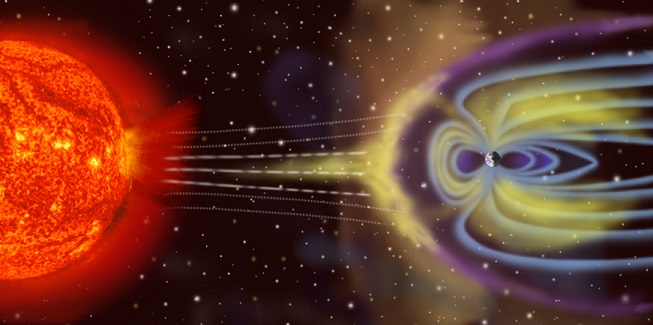
Figure 5. Artist's impression of the solar wind and the earth's magnetosphere (NASA)
We now go even lower in frequency to consider other types of natural electromagnetic phenomena which arise, not from lightning, but from the sun. The sun's surface is a frothing soup of electrically-charged particles, and these continually blow away into space to form the so-called solar wind. When the wind reaches the earth it distorts its magnetic field, compressing it on the sunward side but stretching it out on the leeward side. The distorted field is called the magnetosphere, illustrated in Figure 5. Because the solar wind is continually buffeting the magnetosphere it creates ultra low frequency waves which resonate in the enormous cavity created within, and at the earth's surface the resonances can be detected as exceptionally feeble magnetic disturbances. Two very different types of disturbance are now discussed - Pc1 and Pc3 magnetic pulsations.
Strings of pearls - Pc1 pulsations
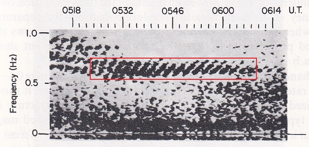
The term 'Pc1' means 'continuous pulsations type 1', minute pulsations in the frequency region around 1 Hz. These can create some remarkable musical sounds if we speed up the radio signal recordings from the receiver to bring them into the audio range. The most fascinating types of signal are called 'pearls' because of their necklace-like visual appearance on a spectrogram (a frequency versus time display). Pearl pulsations were first detected in the mid-twentieth century and an early example is highlighted within the red box on the spectrogram in Figure 6. Although this signal is very noisy a sequence of rising tones or chirps can be discerned, that is, a succession of shorter bursts whose frequency increases with time. Each one arises from an isolated packet of energy travelling within the magnetosphere along a line of the earth's magnetic field, and bouncing back when it reaches the top side of the ionosphere at either end. Careful examination of the picture shows that the slope of each chirp gets less steep as time progresses, so they start to fall over on top of each other towards the end of the sequence. It is important to simulate this feature for musical purposes since it means that the subjective effects vary throughout the Pc1 event.
Figure 6. Spectrogram of a Pc1 'pearl' pulsation event (Troitskaya [8])
As with Schumann resonances, the signal to noise ratio of received Pc1 pulsations is usually poor and therefore unusable for musical purposes. So they were again re-created synthetically, but since their actual frequency lay below 1 Hz they were obviously synthesised at a much higher musical pitch - unlike Schumann signals, their frequency is so low that they cannot sensibly be auditioned at all in real time. The choice of root pitch for the synthetic sample was pretty much immaterial since the frequency of the resulting waveform was interpolated to cover the desired keyboard compass. Since interpolating downwards rather than upwards is more straightforward a reasonably high pitch was preferable. To generate the synthetic signal I used a speed-up factor of 800 so that the mean frequency of the chirps became 523 Hz or treble C (MIDI 72). Chirp bandwidths, time separations and slopes estimated from the spectrogram were all adjusted by the same scale factor. A sequence of 17 chirps was created using the signal generator app in Steinberg's WaveLab audio editing package since this facilitated the necessary layering of the multiple chirp waveforms. The resulting signal sample was synthesised using interpolation over 5 octaves starting at 8 foot C (MIDI 36).
The sound clip below is a sequence of five single notes played at octave intervals starting at tenor C (MIDI 48):
Pc1 - synthesised pearl pulsation - 5 notes 1.46 MB/ 38s
Since the lower pitched notes are of longer duration, the visual features in the spectrogram (Figure 6) can be more easily correlated with what you hear in these cases. In particular, the reduction in chirp slope with time causes the chirps to progressively overlay each other and this causes an echo-like effect to emerge over the signal duration even though no reverberation was added. It adds to the aural spaciousness of the sample, providing a reminder of the vast dimensions of the resonant magnetospheric cavity within which these signals arise in nature. Of course, adding reverberation deliberately can enhance this impression.
The next clip is of three root position C major triads played at successive octave intervals starting at middle C (i.e. with MIDI root Note Numbers of 60, 72 and 84). This is demonstrates that ordinary notated music can be played using 'pearl' sounds if desired:
Pc1- synthesised pearl pulsation - Cmajor chords 766 kB/ 19s
The elusive just minor third - Pc3 pulsations
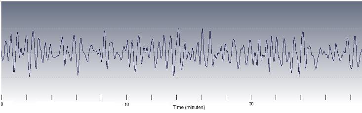
Going still lower in frequency brings us to Pc3 magnetic pulsations ('continuous pulsations type 3') which typically have frequencies around 25 mHz [9]. Since the unit of mHz means 'millihertz' or thousandths of a Hertz, 25 mHz is a frequency of 0.025 Hz or an electromagnetic wave with an oscillation period of 40 seconds for a single cycle. These pulsations arise from extremely low frequency resonances created by the ferocity of the solar wind buffeting against the colossal echoing cavity of the magnetosphere on the sunward (daytime) side of the earth. Pc3's sometimes last for hours and a typical example of the voltage waveform emerging from the receiver is at Figure 7.
Figure 7. Showing about 30 minutes of Pc3 data (Pykett [9])
The signal to noise ratio of this signal was better than those of the Schumann data (Figure 2) and the Pc1 example (Figure 6). This was to a large extent within my control since I designed and built the receiving system and installed it at a remote location at Goonhilly Downs in Cornwall, England far from sources of manmade electromagnetic interference. As a reminder of the exceedingly low frequencies involved, note that the relatively few cycles comprising the waveform segment shown here represent nearly half an hour's worth of data. Although there are some irregularities, the relatively clean waveshape suggests the presence of only a few dominant frequencies rather than wideband noise, and the spectrum in Figure 8 below confirms this.
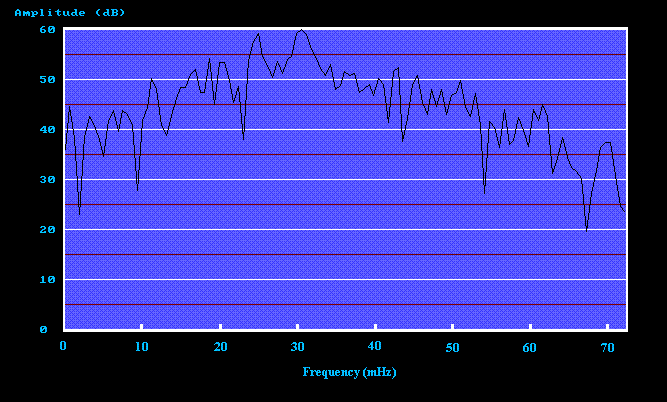
Figure 8. Frequency spectrum of the Pc3 waveform shown in Figure 7 (Pykett [9])
The two principal peaks of equal amplitude at 25 and 30 mHz sit well above the background, and they correspond to separate resonance processes in the magnetosphere. Clearly one would have to speed up the recording by a large factor before these very low frequencies could be heard (e.g. the two dominant frequencies would become 350 and 420 Hz for a speed increase of 14,000). Although this could be achieved easily the practical problem would then become data length - the 30 minute sample depicted in Figure 7, for example, would reduce to only 128 milliseconds. It would also be impossible to loop the sample successfully, both because of its short duration and because of its non-deterministic character. Consequently raw Pc3 data cannot easily be used for musical purposes even if its signal to noise ratio were high enough.
So for the purposes of this article it is more profitable to focus on the two dominant frequencies, 25 and 30 mHz, revealed in the spectrum plot of Figure 8. In musical terms they are 316 cents apart, which is a just (perfectly tuned) minor third in which the frequencies of the two notes form the exact integer ratio 6/5. Assuming the usual pitch standard of A440, the hypothetical physical notes nearest to these two frequencies would lie 13 octaves below the B before middle C (MIDI 59), and the A flat below that (MIDI 56). The interval of a just minor third does not occur in equal temperament (ET) tuning where all minor thirds are considerably flattened or narrowed to 300 cents, thereby contributing to the unpleasant beats of the consonant intervals in ET. It is also rare to find just minor thirds in unequal temperaments, where just major thirds have historically grabbed the focus over the centuries. Kirnberger II is one of the few examples of an unequal temperament boasting a just minor third (two of them). It is therefore remarkable that Nature has provided a rare example of perfect tuning of which the ancient Greeks would have been proud in the principal frequencies of Pc3 pulsations! Their concept of an inaudible Music of the Spheres understandably retains some appeal when viewed against this interconnected background of music, mathematics and physics.
Naturally-occurring audio frequency artefacts caused by lightning such as 'whistlers' have been studied extensively in science, and they have also found a niche in contemporary music of both the serious and popular genres. However the lower frequency manifestations of lightning such as Schumann resonances have attracted less attention from musicians, and the still lower frequencies involved in disturbances originating in the earth's magnetosphere have been largely ignored. This is understandable since these phenomena go deep into the infrasound region, thus they cannot be heard directly. Consequently this article has investigated the possibilities for creating music inspired by Schumann resonances and by ultra low frequency waves below 1 Hz. Aspects of the signals relevant to music have been highlighted, revealing some noteworthy coincidences. For instance, the lowest Schumann resonance at 8 Hz coincides with that of an organ pipe speaking 64 foot C, and the partial structure of Schumann waves is akin to that of church bells. The two therefore sound similar when the Schumann frequencies are translated into the audio region.
It was also demonstrated that Pc1 'pearl' pulsations near 1 Hz produce some remarkable sounds when synthesised at music frequencies, evoking an impression of the vast reverberant cavity of the magnetosphere within which they originate. At still lower frequencies a striking observation was that the two strongest components in the spectrum of Pc3 pulsations formed the interval of a just (perfectly tuned) minor third on A flat. The just minor third is rarely heard in Western music even in unequal temperaments.
All of the phenomena mentioned share the common fascination that they have always been part of the environment in which we have evolved, so the ancient Greek concept of an inaudible Music of the Spheres therefore retains some appeal when viewed against the interconnected background of music, mathematics and physics drawn out in the article. The included audio examples demonstrated the wide range of novel sounds which can be rendered digitally and hence used in music, thereby highlighting some original ingredients which composers and performers can manipulate.
1. For example, see:
https://hackaday.com/2017/11/06/sferics-whistlers-and-the-dawn-chorus-listening-to-earth-music-on-vlf/
(accessed 4 November 2020)
https://space-audio.org/sounds/
(accessed 4 November 2020)
3. Robert Hope-Jones included a 64 foot Gravissima stop in his 1896 organ at Worcester cathedral in England. However it only produced an illusion of such low frequencies (8 Hz at bottom C) because it relied on the beats between two higher frequencies derived from a 32 foot flue pipe rank sounding the interval of a perfect fifth. Since there is no acoustic energy in a beat, the effect of such 'resultant' stops is usually disappointing. Some other organs have incorporated 64 foot reed stops whose resonators at bottom C are indeed 64 feet long, though with reed pipes as opposed to flues, the subjective listening experience at these frequencies is dominated by the extensive retinue of harmonics at higher frequencies rather than at the fundamental itself.
4. Figure 1 is licensed under the Creative Commons Attribution-Share Alike 3.0 unported license (https://creativecommons.org/licenses/by-sa/3.0/deed.en)
5. "Application of the Schumann resonance spectral decomposition in characterizing the main African thunderstorm center", M Dyrda et al, Journal of Geophysical Research: Atmospheres, December 2014.
6. 'A440' means that the frequency of the note A above middle C takes a frequency of exactly 440 Hz which is modern 'concert pitch'. The frequency of the note lying 5 octaves below middle C then becomes 8.2 Hz in equal temperament tuning. This is '64 foot C' in organ terminology, it has a MIDI Note Number of zero, and it is the frequency of the first Schumann resonance mode. These coincidences are very convenient to the digital musician in the context of this article.
7. To avoid the need for real time additive synthesis an alternative approach would have been to pre-compute fully synthesised samples offline and export them to a sound sampler. However, because the Schumann partial frequencies are inharmonic, the resulting summed waveform is aperiodic in that successive cycles are not identical. It is difficult to loop such samples, hence the approach adopted here in which each partial was looped independently and their sum then obtained using real time synthesis. Looping the partials is easy since each is merely a sine wave.
8. "Micropulsations and the state of the magnetosphere", V A Troitskaya, Solar Terrestrial Physics, Academic Press, 1967
9. "The diurnal variation of the polarisation of 25-mHz (Pc3) micropulsations in the horizontal plane", C E
Pykett, Journal of Atmospheric and Terrestrial Physics, 34, 1972.
|