Objective differences between the sounds of baroque and romantic principal
stops
Colin Pykett
Posted:
7 June 2021
Revised: 9 June 2021
Copyright C E Pykett
Abstract. It is not difficult to identify features in the waveforms and spectra of individual organ pipes consistent with subjective assessments of how they sound, but it is more challenging to explain how the many pipes comprising a complete organ stop sound as they do. The problem is important because individual pipes do not make music as generally understood, since organ music is a dynamic aural tapestry woven in real time across the entire rank. Therefore the issue looms large when comparing stops whose pipes are similar yet which sound distinctly different to the ear when music is played on them. The example considered in this article is of this kind, in which two Principal stops from different 'schools' of organ building are studied. One was made by Gottfried Silbermann in Germany in the 1740s and the other by Brindley and Foster in England in the 1900s, and the article includes recordings of traditional organ music made using them to illustrate the point.
One problem addressed is the scatter among the harmonic amplitudes seen in the spectrum of almost any organ pipe, and this leads to another in which the spectra of pipes within a given stop, even adjacent ones, are often grossly different. Yet the ear somehow is able to 'listen through' these major disparities to form a relative judgement of the psycho-acoustic qualia of stops such as those mentioned despite the idiosyncrasies of the data. A further practical difficulty was that when dealing with organ pipe sounds at the level of entire ranks rather than as individuals, the amount of work involved can easily become colossal. Not only is it necessary to study the sounds of many pipes comprising a stop, but one can then drown in the resultant sea of numbers. Information can easily become confused with data, a trap which many fall into. The way this data explosion problem was addressed while keeping the results in focus forms a dominant theme of this article.
The solution adopted was to use only three parameters to represent the acoustic spectrum of individual pipes in the two organ stops studied, rather than the amplitudes and frequencies of all their many harmonics. Without this it would have been impossible to reach any conclusions at all. Using this major simplification, only three graphs were then necessary to demonstrate how the tone quality of each stop varied across the key compass. It was also possible to explain how some aspects of the curves were compatible with the likely scaling and voicing practices applied to each pipe rank by their respective builders, despite the ravages of age, neglect and abuse which the Silbermann pipes in particular must have experienced over nearly three centuries.
These results and the means of deriving them are believed to be original.
Contents
(click on the headings below to access the desired section)
Introduction
Methodology
Results
Silbermann
Principal
Brindley & Foster Open
Diapason
Summary and conclusions
Notes and references
Introduction
Organ aficionadi are well aware that old 'baroque' organs from the time of Bach in the eighteenth century sounded distinctly different to more recent 'romantic' ones. There are many reasons for this to the extent that just listing them all would require an article in itself, so to make progress we need to clear the wood to see the trees. Thus let us reduce matters to a simpler form by considering the following hypothetical situation: for the sake of argument, assume that we have planted two principal (diapason) stops on the soundboard of the same organ, one rank consisting of German pipes from the 1730s (say) and the other representing 1930-ish English ones. Not many players or listeners would confuse them, but why? Many answers to this question would doubtless focus on differences in winding, action, pipe construction, scales and voicing practices, but to my mind this misses the point. We do not hear things like pipe scales and voicing practices; we hear sound waves in the atmosphere. So what is it about the
actual sounds which enable the ear to form such an unambiguous judgement about the type of stop we are listening to? This forms the subject matter of the article.
A difficulty in work of this kind is that one cannot draw useful conclusions from the sounds of individual pipes. Single notes do not constitute music. However, attempts to make sense of the timbres or tone qualities of all the pipes comprising a given stop are made difficult because they fluctuate unevenly from one note to the next
[1]. The subjective verdict of the ear confirms this, and it is precisely these haphazard variations which endow organ stops with much of their charm as the music unfolds. Yet the apparent paradox still remains that stops whose pipes look similar on the face of it, such as the baroque and romantic principals mentioned above, do sound identifiably different despite their variations within each rank - the ear seems to be able to 'listen through' the note-to-note differences when coming to its
judgement. So what features in the sounds is the ear latching onto? I maintain that the question is unanswerable until one adopts an holistic approach which encompasses in some way the sounds of an entire rank of pipes rather than focusing on individual ones, yet without the method becoming so generic that the differences between ranks get obscured or averaged out. We must not throw the baby out with the bath water. Unfortunately, in following this approach a further, practical, problem then raises its head. If we have to deal with organ pipe sounds at the level of entire ranks rather than as individuals, the amount of work involved can become colossal if we are not careful. Not only is it necessary to record the sounds of each pipe comprising a stop (expensive, difficult and time consuming in itself), but back in the lab we can then drown in the resultant sea of numbers. We can so easily confuse information with data, a trap which many fall into. Hence the way I have addressed this data explosion problem while keeping the results in focus is a dominant theme of this article.
Methodology
Recordings were made of the same piece played on the main 8 foot Principal or Diapason stops on two different organs. The piece chosen was the chorale melody
'Freu' dich sehr, o meine seele' by G Kauffmann as harmonised by J S Bach in movement 7 of his cantata BWV 70. One of the organs was made by Gottfried Silbermann in Germany in the early 1740s and the other by Brindley and Foster in England in the early 1900s. In both cases the pipe sounds had previously been sampled (recorded note by note) and subsequently rendered by my
Prog Organ virtual pipe organ.
The Silbermann organ stood in a fairly compact building with a correspondingly short reverberation time and the pipe sounds were
close-miked during sampling. Therefore the recording here sounds fairly dry, pretty much as it would to a listener seated relatively close to the actual instrument. This enables the detail and subtlety of the original sounds to be reproduced without being swamped by the acoustic of the building. The organ spoke about a semitone above today's usual pitch (A440) and it was tuned to equal temperament, or something close to it, rather than to the sixth-comma meantone tuning sometimes used by
Silbermann:
 BWV 70/7 played on a Silbermann Principal - 1m 12s/1.1 MB
The Brindley and Foster organ was in a larger building but the samples were again
close-miked to avoid losing too much detail. This instrument was tuned to A440 in equal temperament:
BWV 70/7 played on a Brindley & Foster Open Diapason - 1m 18s/1.2 MB
Although the Brindley stop was made more than 150 years after the Silbermann one and represents a quite different organ building tradition in a distant country, it stands well clear of the opaque excesses of tone which characterised the nadir of the romantic movement in England at that time. This is because the tonal concept and execution of Brindley's organs, like those of Lewis, were influenced by the nineteenth century work of Edmund Schulze in Britain, and in turn the tonal roots of Schulze's work were affected by what he had inherited in craft and tradition from builders such as
Silbermann. So although we might regard B & F's organs as ostensibly romantic, one can trace an admittedly tenuous thread from Silbermann through to them. Nevertheless it is not difficult to perceive distinct differences between the sounds of the two stops in these recordings. The Silbermann Principal 'chuffs' almost explosively onto speech, though without hissing and spitting in the unpleasing way that some neo-baroque organs of the twentieth century tended to do. However these attack transients are largely absent in the Brindley stop, which also conveys an impression of greater smoothness and constancy in regulation (volume from note to note) across the rank. At this remove in time it is difficult to say whether these features in the sounds have resulted more from the many vicissitudes to which the much older Silbermann organ must have been subjected, or whether he chose to leave his fluework in this arguably more characterful state in the first place.
The attack transient of a flue pipe, if present, usually consists of a short burst of sound containing both tonal and noise-like elements. The noise arises from the often turbulent air jet passing through the flue slit between the lower lip and the languid and then impacting the upper lip. The evanescent musical tones arise because the sudden inrush of air into the pipe body fleetingly excites its natural
resonances, in much the same way that dropping a knife onto a dinner plate makes it 'ring' briefly. Like those of bells, these resonances or partials are inharmonic, meaning that their frequencies bear no simple numerical relationship one to another. This is unlike the harmonics emitted when the pipe speaks steadily during its subsequent sustain phase, when each harmonic is an integer (whole number) multiple of the fundamental frequency. Therefore, during the brief attack transient, the inharmonic partials get progressively pulled into phase-lock to become the exact harmonics of the sustain phase. So if pronounced partials are generated during an attack transient, it is often the case that the corresponding harmonics which they morph into are also prominent. Consequently we might expect the Silbermann stop with its noticeable transients to also show evidence of stronger harmonic development in the sustain phase than the Brindley one, at least for some pipes. If so, this would influence its timbre or tone colour as well. So this is one route we might follow when trying to relate subjective aspects of the two stops to objective measurements of the pipe sounds.
But how do we assemble the evidence concerning the timbre of an entire organ stop over all the pipes in a rank? The first step is to find a means of capturing the essentials of the harmonic structure of a single pipe, its frequency spectrum, using just a handful of numbers rather than the surfeit of data which the spectrum itself contains in the amplitudes and frequencies of all its harmonics. These numbers must not be unduly influenced by the spectral scatter which occurs among the harmonic amplitudes of an organ pipe in practice, nor by the haphazard changes which occur from one pipe to the next. These matters are expanded in what follows.
Results
The aspects discussed above will be illustrated by referring first to Silbermann's Principal stop.
Silbermann
Principal
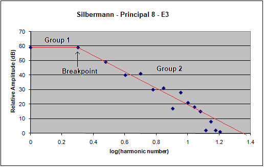
Figure 1. Spectrum of a Silbermann Principal pipe (middle E). Two trendlines are also shown.
The blue dots in Figure 1 show the harmonic spectrum of the middle E pipe (E above middle C) from Silbermann's Principal rank, showing the scatter among the points which typifies that observed with organ pipe spectra. Observe that the pattern of harmonics falls naturally into two regions labelled Group 1 and Group 2, which have been associated with the two trendlines drawn on the graph. It is remarkable that a two-group structure is common to virtually all of the organ pipe spectra I have examined over several decades of research, embracing flute, diapason, string and reed pipes
[2]. The two lines intersect at a point which is called the 'breakpoint' here, and the two lines can be used to represent the complete spectrum instead of using all its harmonics.
The justification for using a trendline approximation to represent a spectrum is that no two pipe spectra across a rank are exactly the same, even adjacent ones. Therefore there is no such thing as 'the sound' of an organ pipe in practice in the sense of it being unique or invariant across a rank. It is this intrinsic variability which enables trendlines to capture the essentials of spectra which are subject to these often major perturbations, because the lines themselves are not influenced as strongly as are the individual harmonics by random variations. The lines tend to 'iron out' the random scatter among the harmonics. Another important feature of trendlines is that they enable a spectrum to be represented using only three numbers in this case - these are the breakpoint or harmonic number at which the two lines intersect, and the slopes of each line measured in decibels per octave. Thus the entire spectrum in Figure 1 was captured by the simple number triplet 2, 0, -18. Respectively, these are the values 2 for the breakpoint expressed in terms of harmonic number, 0 dB/octave for the slope of the Group 1 trendline and -18 dB/octave for the Group 2 slope. This representation is far more economical than the 32 numbers which would otherwise have been required (the amplitudes and frequencies of 16 harmonics) and therefore it is much easier to handle. Thus we have gone some way towards solving the problem posed earlier - how to represent the essentials of the harmonic structure of an organ pipe using just a handful of numbers.
However the question actually posed was much bigger than this - how do we assemble the numerical evidence concerning the timbre of an entire organ stop over all the pipes in a rank? Consequently the next step requires the spectra, now represented economically in the form of number-triplets, to be related to the timbre or harmonic structure of the stop across its whole compass. This was done as follows. The spectra of thirteen pipes equally spaced across the first four octaves of this Principal rank (three per octave plus top C) were computed, and trendlines were derived for each one. In each case the three numerical values defining the two lines were then plotted in terms of their position in the key compass. This resulted in the three graphs shown in Figure 2, one for each trendline parameter (the breakpoint and the two trendline slopes). The horizontal axis of each graph represents physical note number running from 1 (bottom C) to 49 (top C). As a final step, best-fit curves (the black lines) were superimposed on each graph in an attempt to reveal overall trends in the data.
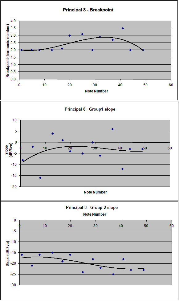
Figure 2. Silbermann Principal - variation of trendline parameters across the key compass
Given the exasperatingly crazy fluctuations frequently seen in organ pipe spectra, the breakpoint curve (top graph) is remarkably well behaved over the first five data points. These cover the bass region of the compass between bottom C and E a major tenth above it, a span of nearly 1.5 octaves. Having a breakpoint value of 2, the Group 1 harmonics (those bounded by the fundamental and the breakpoint) therefore include only the first two harmonics over this note range, as in the example spectrum in Figure 1. Beyond this however, the best-fit curve shows an average increase towards 3 over the central region of the compass, though there are considerable fluctuations either side of this value. This suggests that the third harmonic moves from Group 2 into Group 1 as one goes higher up the keyboard, but the effect tails off again in the top octave where the behaviour reverts to that seen in the bass where Group 1 comprises only the fundamental and second harmonic.
The first five data points of the Group 1 trendline slope (middle graph) show its value varying markedly from note to note, though the best-fit curve is less affected. This is because the third point is an obvious outlier compared with the trend of the others. So, on average, the best-fit curve shows the Group 1 trendline slopes of the pipes rising from -8 dB/8ve at bottom C (sloping strongly downwards) to -2 dB/8ve (more nearly horizontal) by the middle of the second octave. Thus these data taken together indicate two main features over this bass key range - firstly Group 1 includes only two harmonics, and secondly the Group 1 trendline becomes progressively less steep above bottom C. These observations suggest that, again on average, the second harmonic of the pipe becomes stronger relative to the fundamental as one ascends from bottom C over the first 17 notes or so, to become much the same as the fundamental by the middle of the second octave.
As to the behaviour over the remainder of the compass, there is still a good deal of scatter among the data points for the Group 1 trendline slope. However the best-fit curve shows that this is largely random in that the average value does not deviate nearly as much (i.e. the Group 1 slope remains roughly where it had got to by the middle of the second octave). This means that the levels of the fundamental and second harmonic remain broadly comparable over the rest of the compass. Together with the result for the breakpoint variation mentioned above, the third harmonic also gets stronger higher in the keyboard until the top octave is reached, whereupon it falls off again.
For the Group 2 trendline slope data (lower graph in Figure 2), the best-fit line suggests that, on average, it gets steeper over the key compass from a value around -17 dB/8ve in the bass to about -22 dB/8ve in the treble. Referring back to the example spectrum in Figure 1 will show that a steeper Group 2 slope means fewer high-order harmonics in the sounds, implying that the treble pipes will have less harmonic development than the bass in this case. In other words, the trebles will be less inclined to scream while the bass will not become too woolly. These are highly desirable characteristics of a flue pipe rank, and it is quite possible that we are seeing Silbermann's fabled scaling practices at work in this graph. This is because pipe scale (the ratio of diameter to length) influences the number of harmonics in the spectrum - narrow scales produce more harmonics than wide scales, other things being equal.
It has taken a lot of words to describe the complexities of these graphs and it would not be surprising if you were little the wiser having read this far. So a more concise summary is called for. In broad terms:
Lowest 1.5 octaves - the 2nd harmonic amplitude increases from bottom C to become comparable with the fundamental by the middle of the 2nd octave.
Central region - this behaviour is maintained, together with a progressive rise in the 3rd harmonic amplitude in addition. Ascending from the bass, the pipes also tend to emit progressively fewer harmonics in total. However these trends are associated with considerable scatter among the notes
analysed, which might have resulted more from the chequered history of this very old pipework rather than from intent on the part of the builder.
Top octave - the 3rd harmonic falls off again, leaving only the fundamental and 2nd harmonic with comparable amplitudes, as in the bass.
These conclusions are convincing in that they accord with the subjective features of the sound of the Silbermann stop. The 'chuffy' attack transients on the recording, so prominent in the middle of the keyboard, arise from inharmonic second and third partials which have faster rise times than the first. So when these partials morph rapidly to become the second and third harmonics of the sustained sound of the pipe, they retain significant amplitudes comparable with the fundamental. It is probably Silbermann's high wind pressures (typically 95 mm of water even in his small organs) which are largely responsible for this
behaviour. Flue pipes winded at this sort of pressure are overblown in the sense that attack transients are likely to be prominent, together with strong early (Group 1) harmonics while the pipes speak. In the analysis presented here this has been reflected both in the audio clip and in the frequency spectra of the pipes as revealed in Figure 2.
Brindley & Foster Open Diapason
We now turn to the Brindley & Foster Open Diapason stop. Graphs in the same format as those for the Silbermann example are shown in Figure 3, except that in this case a few more data points were available for each graph because the Brindley stop was of full five octave compass, enabling additional spectra to be analysed at the top end.
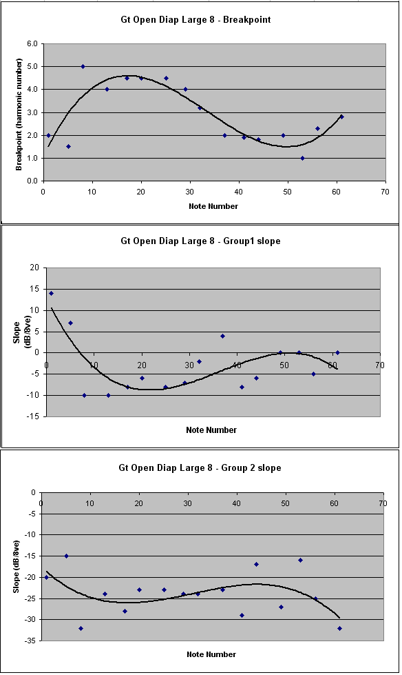
Figure 3. Brindley & Foster Open Diapason - variation of trendline parameters across the key compass
At first glance the two data sets in Figures 2 and 3 look appreciably different, and presumably this reflects in some way the aural dissimilarities between the two stops heard on the recordings. However, more detailed analysis is necessary before this statement and more detailed underlying relationships can be confirmed. Firstly consider the slopes of the Group 2 trendlines as plotted in the lower graph. These lines are associated mainly with the high order/lower amplitude harmonics in each pipe spectrum as shown earlier by Figure 1, and the best-fit curve suggests that their slopes end up steeper in the treble than where they started in the bass. This behaviour is qualitatively similar to that of the Silbermann Principal. However most of the numerical values here are noticeably lower than in Figure 2, meaning that the trendline slopes are, on average, somewhat steeper across the key compass. This implies that the sounds of the Brindley Diapason pipes contain rather fewer higher harmonics than the Silbermann Principal. This is not unexpected for a stop from the romantic era.
Nevertheless, in both cases the data therefore suggest that more harmonics will be emitted by the bass pipes, where the Group 2 line slopes are less steep, than in the treble where the reverse applies. This is precisely the behaviour encouraged by a sensible scaling law, such as that also used by
Silbermann, which makes the bass pipes narrower relative to their speaking length compared with pipes in the middle of the compass. Narrower pipes emit more harmonics, other factors being equal. Towards the treble the scaling law makes the pipes wider relative to their length and thus they emit fewer harmonics, a feature suggested by the Group 2 graphs for both stops. It is therefore credible that this graph is reflecting much the same spectral, and thus tonal, variations across the key compass which make the Brindley scaling law qualitatively (if not numerically) similar to that of the Silbermann stop discussed above. However one must also take into account deliberate shading effects introduced by the respective voicers across these two ranks, since tonal finishing (including winding adjustments) as well as scale contribute to the overall effect of any organ stop. On the other hand, effects due to pipe scale will survive over time far better than those due to voicing since pipes will retain their scale regardless of what history might do to them, whereas this is certainly not true of voicing and regulation where every interventionist will have been unable to resist meddling with them. This will be particularly relevant to the chequered and largely undocumented history of the much older Silbermann pipes. It is not really possible to take the discussion much further, beyond reiterating that both stops seem to lose their high frequency edge towards the treble in ways hinted at by these graphs.
The other two parameters in Figure 3, the breakpoints and the slopes of the Group 1
trendlines, show an interesting feature towards the bass end of the compass which was not seen in the Silbermann stop. For the Brindley rank the breakpoint value decreases markedly, whereas simultaneously the Group 1 slope changes rapidly from a negative value to a positive one. Taken together, these result in significant changes in the spectra towards the extreme bass. Higher in the compass a typical spectrum shape for a principal or diapason pipe was shown in Figure 1, whereas in the bottom octave it becomes quite different for the Brindley stop. To illustrate this, the spectrum for the bottom note is shown in Figure 4 below.
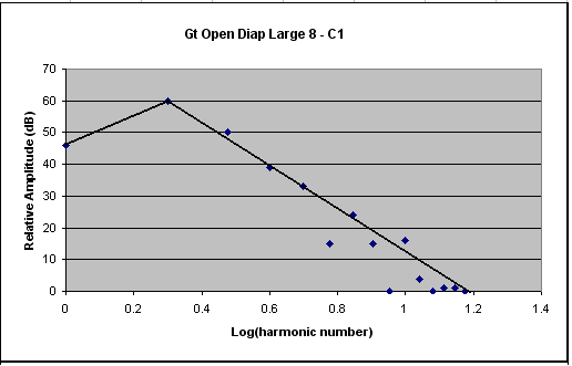
Figure 4. Spectrum of a Brindley & Foster Open Diapason pipe (bottom C). Two trendlines are also
shown
Notice how the Group 1 trendline now has a steep positive (upwards) slope, whereas the middle graph of Figure 3 shows that it was negative (downwards) over most of the key compass. The breakpoint has also reduced from its former value to lie at the second harmonic (top graph, Figure 3). These changes result in this pipe emitting a second harmonic of much higher relative amplitude than those further up the keyboard, and this also applies to some of the subsequent harmonics. For this pipe the second harmonic has reached five times the amplitude of the fundamental (14 dB), and even the third harmonic is about 1.6 times stronger (4 dB). This is quite different to many pipes higher in the compass where the strongest harmonic is the fundamental itself. This behaviour results in the bass pipes of this diapason stop sounding much brighter and less ponderous than they would otherwise have done had no scaling been applied. This is partly a consequence of the relative narrowing of the pipes towards the bass, therefore the data here might again be reflecting tonal characteristics related to the scaling of this rank. However these effects could also have been emphasised by rather dramatic voicing and perhaps winding adjustments over the bottom few notes, as discussed earlier. It is not easy to say which effect predominates here - pipe scale or voicing - purely from an examination of these data, though both will undoubtedly have played their part.
As a final observation concerning the Group 1 slope data (middle graph), the Brindley curve exhibits noticeably less point-to-point scatter than the corresponding one for the Silbermann stop over most of the compass above the extreme bass. This might partly account for the subjectively 'smoother' aural effect noticeable on the Brindley recording. However it is impossible to say whether the difference can be related to original intent on the part of Silbermann or whether it merely reflects the vicissitudes of fortune which these very old pipes will have experienced. For what it is worth, I find it difficult to accept that a builder of Silbermann's reputation would have left his pipework in the rather slapdash state implied by the Group 1 data in Figure 2. It seems more plausible, and respectful, simply to write it down to the history and old age of this venerable stop.
Summarising in broad terms the observations above for the Brindley & Foster stop:
Lowest few notes - the 2nd and 3rd harmonics in this region of the compass suddenly become significantly stronger than the fundamental or any other.
Remainder of the compass - the fundamental becomes the dominant harmonic in most cases. Ascending from the bass, the pipes also emit progressively fewer harmonics. The low-order harmonics (those in Group 1) exhibit less scatter than the Silbermann Principal, probably resulting in more aural 'smoothness' and constancy in regulation (volume from note to note) across the
rank.
Summary and conclusions
It is not difficult to discover and quantify features in the waveforms and spectra of individual organ pipes consistent with subjective assessments of how they sound, but it is far more challenging to explain how a rank of many pipes comprising a complete organ stop sounds as it does. The problem is important because individual organ pipes do not make music as generally understood, thus it looms large when comparing stops whose pipes are similar yet which sound distinctly different to the ear when music is played on them. The example considered in this article was of this kind, in which two Principal stops from different 'schools' of organ building were studied, and the article included recordings made using them.
A problem which had to be addressed is the inherent scatter among the harmonic amplitudes seen in the spectrum of almost any organ pipe, and this led to another in which the spectra of the pipes within a given stop, even adjacent ones, are often grossly different. Yet the ear somehow is able to 'listen through' these major disparities to form a relative judgement of the psycho-acoustic qualia of stops such as those mentioned despite the inadequacies of the data. A further difficulty was a practical one - in dealing with organ pipe sounds at the level of entire ranks rather than as individuals, the amount of work involved can easily become colossal. Not only is it necessary to study the sounds of many pipes comprising a stop, but one can then drown in the resultant sea of numbers. Information can so easily become confused with mere data, a trap which many fall into. The way this data explosion problem was addressed while keeping the results in focus formed a dominant theme of this article.
The solution adopted was to use only three parameters to represent the acoustic spectra of individual pipes in the two organ stops studied, rather than the amplitudes and frequencies of all their many harmonics. Without this it would have been impractical to reach any conclusions at all. Using this major simplification, only three graphs were then necessary to demonstrate how the spectra and thus the tone quality of each stop varied across the key compass. It was also possible to explain how some aspects of the curves were compatible with the likely scaling and voicing practices applied to each pipe rank by their respective organ builders, notwithstanding the ravages of age, neglect and abuse which the Silbermann pipes in particular must have experienced over nearly three centuries.
These results and the means of deriving them are believed to be original.
Notes and references
1.
The random variations from note to note are superimposed on the systematic ones which occur across a rank owing to the effects of pipe scales and voicing adjustments.
2. "Some novel observations on organ pipe sounds and their frequency
spectra", C E Pykett, November 2015, an article on this website.